Instructional Software for Reliability Estimation and Fault Tree Analysis

(1)

Instructional Software for Reliability Estimation And Fault Tree Analysis

Rashpal Ahluwalia

Department of Industrial & Management Systems Engineering, West Virginia University

Morgantown, WV 26506

Corresponding author’s Email: [email protected]

Author Note: Dr. Ahluwalia is professor of Industrial and Management Systems Engineering at West Virginia University, Morgantown, WV. His areas of interest are Manufacturing, Information Technology, Quality, and Reliability Engineering. Dr. Ahluwalia is fellow of the American Society for Quality (ASQ), a life senior member of the Institute of Electrical and Electronics Engineers (IEEE), a registered Professional Engineer (PE) in West Virginia, and ASQ Certified Software Quality Engineer (CSQE). The author would like to acknowledge contributions of Mr. Mitesh Parekh and Mr. Chihui Li towards reliability software implementation.

Abstract: This paper describes a software tool to introduce fundamental concepts of reliability and fault tree analysis to engineering students. Students can fit common failure distributions to failure data. The data can be complete, singly censored, or multiply censored. The software computes distribution and goodness-of-fit parameters. The students can use the tool to validate hand calculations. Failure distributions and reliability values for various components can be identified and stored in a database. Various components and sub-systems can be used to build series- parallel or complex systems. The components data can also be used to build fault trees. The software tool can compute reliability of complex state independent and state dependent systems. The tool can also be used to compute failure probability of the top node of a fault tree. The software was implemented in Visual Basic with SQL as the database. It operates on the Windows 7 platform.

Keywords: Connection Matrix, Tie-set, Cut-set, Failure Distributions, Statistical Tests, Fault Tree, Reliability, Software, Markov

1. Introduction

On March 11, 2011, Japan was hit by a magnitude 8.9 earthquake which occurred underwater at a depth of 20 miles, about 40 miles east of Oshika Peninsula. The earthquake triggered tsunami waves up to 128 feet, resulting in massive destruction and loss of over 14,000 lives and 10,000 missing. In addition to loss of life, at least three nuclear reactors suffered explosions after their cooling systems failed. Radiation levels at the Fukushima No. 1 nuclear plant were reported to be 1,000 times normal (Magnier, 2011). The U.S. Nuclear Regulatory Commission is now examining the safety and reliability of its 104 nuclear plans.

There have been several other major disasters, such as the explosion of the space shuttle Challenger on January 28, 1986, caused by the failure of O-rings that were used to seal the four sections of the booster rocket. On March 28, 1979, there was a partial core meltdown at the Three Mile Island nuclear power plant. It was caused by a stuck-open relief valve which allowed nuclear reactor coolant to escape. On April 26, 1986, there was a complete core meltdown at the Chernobyl nuclear plant (Schlager, 1994). Each accident was a result of unique circumstances, caused either by nature, hardware/software malfunction, human error, or a combination.

In order to determine reliability and safety of a complex system, such as a nuclear power plant, one needs to identify all of its critical sub-systems and components. Typically, it takes several software tools to analyze failure data, identify failure distribution(s), parameter estimation, component reliability analysis, estimation of reliability of state independent and state dependent systems, and fault tree analysis. This paper describes a software tool that integrates these tasks and can be used to teach fundamental concepts of safety and reliability engineering.

The literature uses various terminology and techniques to estimate component and system reliability. This paper defines a system to be made up of several sub-systems and components. A sub-system consists of other sub-systems and components. A component is defined as an entity that cannot be further divided. A sub-system or a component is called an

item. A system and a sub-system are essentially the same. Scope of a given study defines a system, for example, the electrical system of an automobile could be studied as a system or a sub-system.

The techniques for evaluating system reliability are based on conditional probability analysis, network reduction, identification of tie-sets and cut-sets, logic diagrams, tree diagrams, and Markov analysis. These techniques can be applied

(2)

for analysis of components, sub-systems, or systems. Probability based analysis is often used to estimate component reliability. It deals with collecting failure data and fitting an appropriate distribution to it, from which the probability of failure during a given time interval can be computed. However, when it comes to system reliability, different techniques are used for different systems.

A series-parallel system is good for the application of network reduction because it does not require intensive calculation. A complex system, which cannot be broken down to a series-parallel system, tie-set and cut-set approaches are appropriate. Markov analysis is suitable for state dependent systems, where failure of an item is dependent on failure of another item. Most commercially available software tools use the tie-set and cut-set approach to estimate system reliability.

2. Reliability Overview

If T is the life of a system, sub-system, or a component, then reliability (R) is defined as the probability that it will not fail during time t, where t ≤ T. Military handbook (1990) defines reliability as the probability, at a given confidence level, that the an item will perform its intended function, for a specified mission time (t), without failure, when used for the intended purpose under the intended operational conditions. The unreliability (F) is the probability that an item will fail during time t. Failures can occur due to wear, corrosions, defects, etc. Reliability and unreliability can vary with time, R(t)

typically decreases with time and F(t) typically increases with time. At any time t, the sum of R(t) and F(t) is 1. Hazard function h(t) is defined as the limit of the failure rate as Δt approaches zero. That is, hazard function is the instantaneous failure rate, it is a conditional probability that the item will fail during time interval [t, t+Δt], given that it did not fail until time t. The cumulative hazard function H(t) is the conditional probability of failure during the time interval [0, t]. The Equations (1), (2), and (3) describe the R(t), h(t), and H(t), respectively.

1 (1)

∆ → _∆ ∆ ∆ ∆ (2)

(3) where 0 < t <+∞, 0 ≤R(t), F(t) ≤ 1, R(0) = 1, F(0) = 0, R(t)t→∞ = 0, and F(t)t→∞ = 1

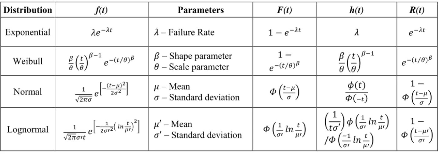
The most commonly used failure distributions for reliability estimation are: The Exponential, the Weibull, the Normal, and the Lognormal. Exponential distribution is used to estimate reliability of hardware items with constant failure rate during their useful life (Ebling, 2005). Many electronic components, such as transistors, resistors, and integrated circuits follow this distribution. Mean time between failures (MTBF) is the arithmetic mean (average) time between failures of a system. It is typically part of a model that assumes that the failed item is immediately repaired (zero elapsed time), as part of a renewal process. This is in contrast to the mean time to failure (MTTF), which measures average time between failures with the modeling assumption that the failed item is not repaired. The scale parameter (λ) of the Exponential distribution is equal to the failure rate (1/ MTBF or 1/MTTF). The Weibull distribution is an approximate model of time to failure if the item is of a type in which a large number of flaws exist (Ebling, 2005). The two parameter Weibull distribution has shape (β), and scale (θ) as its parameters. The normal probability distribution function is used to model failures due to fatigue or wear out. The parameters of the normal are its mean (μ) and variance (σ2_{). The normal is not a true reliability distribution} since the random variable ranges from minus infinity to plus infinity. The positive portion of the normal does provide a reasonable approximation to the failure process. The dispersion about the mean is dependent on the value of the variance or standard deviation. The Lognormal distribution is a good model for times to failure when failures are caused by fatigue cracks. The Lognormal is defined only for the positive values of t and is more appropriate than the Normal distribution as a failure distribution. Like the Normal, it has μ′ as the scale parameter (or median) and σ′ is the shape parameter. Table 1 shows f(t), parameters, F(t), h(t), R(t) functions for the above failure distributions.

(3)

Table 1: Common Failure Distributions

Distribution f(t) Parameters F(t) h(t) R(t)

Exponential – Failure Rate 1

Weibull ⁄ – Shape parameter

– Scale parameter 1 ⁄ ⁄ Normal √ – Mean – Standard deviation 1 Lognormal √ ′– Mean ′ – Standard deviation 1 ′ / 1

2.1 Failure Distribution Selection

The first step in identification of candidate failure distributions is collection of failure data. There are basically two types of failure data, complete data and censored data. Complete data is when time to failure of all items is available. Censored data can be single or multiply censored. Type I single censored data is when testing is terminated after a fixed length of time. Type II single censored data is when testing is terminated after a fixed number of failures. In multiply censored data test times differ among censored items. After failure data is collected one needs to identify candidate distributions, estimate distribution parameters, and perform goodness-of-fit test. Least squares technique is often used to fit a curve to the failure data. The least squares regression equation is given by (4). The coefficient of determination given by (5) is used to measure the strength of fit. The square root, r, is the index of fit, its value is between -1 and 1; a value | | of 1 indicates a perfect fit.

y ∑ x β i = 1, 2, …, m (4)

Where, m = number of linear equations, n = number of unknown, m > n, and β1, β2, …, βn are regression coefficients.

1 ∑_∑ (5)

Table 2 shows the transformation of failure data for the least squares model for the four common distributions, where F(ti) = (i-0.3) / (n+0.4). This formula is used as an approximation of the median position. Once the distribution is

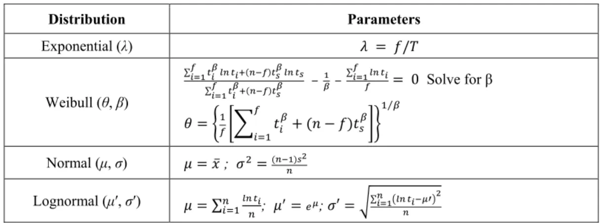
known, the next step is to determine its parameters. There are several approaches to parameter estimation. Table 3 shows the Maximum Likelihood Estimation (MLE) equations for parameter estimation for the four common distributions. The final step is to perform a statistical test for goodness-of-fit. This test compares the null hypothesis (H0: The failure times come from the specified distribution) to the alternative hypothesis (H1: The failure times do not come from the specified distribution). The test consists of computing test statistic, which is compared to the critical value. The critical value is based on the level of significance (α) of the test and the sample size. Different tests are available for different distributions. For instance, Kolmogorov-Smirnov test is used for normal and lognormal distributions, Bartlett’s test is used for the exponential distribution, and Mann’s test is used for the Weibull distribution. These specific tests are more powerful than the general Chi-square test. The Goodness-of-fit test equations for the four basic distributions are shown in Table 4.

(4)

Table 2: Least square approach for common distributions Distribution x i yi Parameters Exponential λ = b Weibull β = b; θ = exp(-a/β) Normal σ = 1/b; μ = -a/b Lognormal σ′ = 1/b; μ′ = exp(-σ′a)

Table 3: MLE approach for common distributions

Distribution Parameters Exponential (λ) / Weibull (θ, β) ∑ ∑ ∑ 0 Solve for β ⁄ Normal (μ, σ) ̅ ; Lognormal (μ′, σ′) _∑ _; _; _′ ∑

Table 4: Goodness-of-fit tests for common distributions

Distribution Formulas Accept H0 If

Bartlett’s Test (B) for Exponential distribution

⁄ ∑ ⁄ ∑

/ ⁄ , ⁄ ,

Mann’s Test (M) for Weibull distribution ∑ ⁄ ∑ ⁄ ; ; 1 . . , , , Kolmogorov-Smirnov Test (D) for Normal/Lognormal distribution ̅ ∑ ; ′ ∑ ̅ ̅

2.2 State Independent Systems

State independent systems are a collection of items where failure of one item is independent of failure of other items. A state independent system can have several configurations. Reliability of a system for a given configuration can be

(5)

determined by applying the combinational rules of probability. Figure 1 shows a series system consisting of n items. System reliability (Rs) of a series system is given by equation (6), where Ri = Reliability of the ith item.

Rs R1 *R2 … *Ri … *Rn (6)

Figure 1: An n item series system

Figure 2 shows an n item parallel system. Reliability (Rs) of a parallel system is given by (7).

Rs = 1 – [(1 – R1)*(1 – R2)… *(1 – Ri) …*(1 – Rn)] (7)

Figure 2: An n item parallel system

A k-out-of-n system is similar to a parallel system where the system survives only if k-out-of-n items survive. The reliability (Rs) of a k-out-of-n system is given by equation (8).

∑ _! ! _!∗ ∗ 1 for k ≤ n (8)

Items of a system can also be configured in series and parallel. Such systems are referred to as series-parallel systems. A five item series-parallel system is shown in Figure 3, with reliability value of each item shown in parentheses. A series-parallel system can be reduced to a series or a parallel system by repeatedly applying equations (6) and (7). Figure 4 shows formation of item X34 from items X3 and X4. Figures 5 shows formations of item X1,34. Figure 6 shows the reduction of the series-parallel system to a simple series system.

Start X1 X2 Xi Xn End

……

X1 X2 Xi Xn End Start

(6)

Start X2 (0.8934) X3 (0.6985) X4 (0.993) End X1 (0.93) X5 (0.98) 1 2 3 4

Figure 3: A five item series-parallel system

Start X34 (0.99789) End X1 (0.93) X5 (0.98) X2 (0.8934) 1 2 3 4

Figure 4: Formation of item X34

Start X1,34 (0.928037) End X5 (0.98) X2 (0.8934) 3 4 1

Figure 5: Formation of item X1,34

Start _(0.992329)X2,1,3,4 X5 End

(0.98)

3 4

1

Figure 6: Reduction to a simple series system

A complex system is a system that cannot be reduced to a simple series or a parallel system. A five item complex system is shown in Figure 7. Reliability of such systems is computed by using techniques such as: tie-sets and cut-sets, event trees, or fault trees. A tie-set is defined as a set of items whose functioning ensures that the system will function. A minimal tie-set (path) is one in which all of the items in a tie-set must function in order for the system to function. A cut-set is a set of items which when fail, result in system failure. A minimal cut-set is one in which all of the items of a cut-set must fail in order for the system to fail. An event tree is a pictorial representation of all the events that can occur in a system. Tie-sets and cut-sets and can be developed from event trees (Singh, 1977). Fault tree is a top-down, deductive analysis technique to identify scenarios for which a particular fault or an undesired event may occur.

(7)

Figure 7: Five item complex system

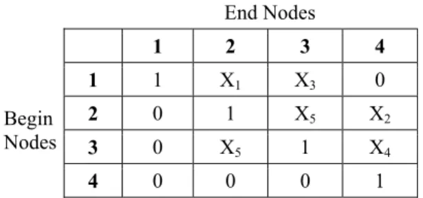
Users often have to use a variety of tools for: a) Analysis of failure data, b) selection of failure distributions, c) Estimation of distribution parameter, d) Network reduction, e) Tie-set/cut-set identification, f) Markov analysis for state dependent systems, and g) Fault tree analysis. Before utilizing any of the tools, the user must identify all of the items of the system and their interconnections. Item interconnections or the Reliability Block Diagram (RBD) can be expressed in a verity of ways for computer based analysis. The most common approach is to use a connection matrix. Table 5 shows a connection matrix for the five item complex system shown in Figure 7. The rows and columns of the connection matrix refer to the begin node and end node of an item. A "1" in the connection matrix indicates that begin node and end node are the same. A “0” value indicates there is no item between the begin node and the end node. Given the connection matrix, minimal tie-sets and cut-sets have to be computed. The minimal tie-sets for the system shown in Figure 7 are shown in Table 6.

Table 5: Connection matrix for the five item complex system End Nodes 1 2 3 4 Begin Nodes 1 1 X1 X3 0 2 0 1 X5 X2 3 0 X5 1 X4 4 0 0 0 1

Table 6: Tie-sets for the five item complex system

NO. Tie-set

T1 X1, X2 T2 X3, X4 T3 X1, X5, X4 T4 X3, X5, X2

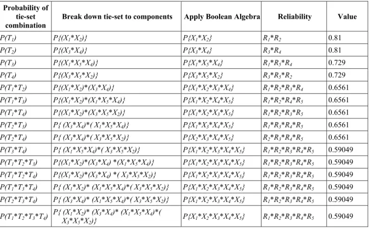
Reliability of the system can be computed by summing the probability of each tie-set as shown in equations (9) and (10). If the reliability values of individual items in Figure 7 were assumed to be .9, then equations (11)-(14) show the values of the intermediate terms. Table 7 shows the reliability values of various combinations of tie-sets. The overall reliability of the system shown in Figure 7 is given by equation (15).

(9) X1 X2 X3 X4 X5 1 3 4 2 Start End

(8)

∗ ∗ ∗ ∑ ∑ ∑ ∑ ∗ ∗ ∗ (10) ∑ = 0.81 + 0.81 + 0.729 + 0.729 = 3.078 (11) ∑ ∑ ∗ ∗ ∗ ∗ + ∗ ∗ ∗ = 0.6561 * 5 + 0.59049 = 3.87099 (12) ∑ ∑ ∑ ∗ ∗ ∗ ∗ ∗ ∗ ∗ ∗ ∗ ∗ = 4 * 0.59049 = 2.36196 (13) ∑ ∑ ∑ ∑ ∗ ∗ ∗ ∗ ∗ ∗ = 0.59049 (14) Rs = 3.078 - 3.87099 + 2.36196 - 0.59049 = 0.97848 (15)

Table 7: Reliability of various tie-set combinations for the five component complex system

2.3 System Representation and Simplification

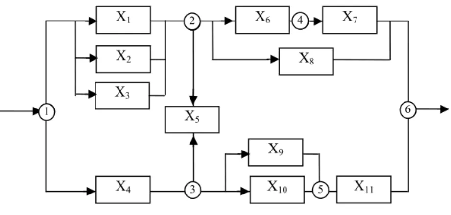
A slightly more complex system with eleven items and nine nodes is shown in Figure 8. The corresponding connection matrix is shown in Table 8. Tie-sets for this system are shown in Table 9. If reliability values of individual items

Probability of tie-set combination

Break down tie-set to components Apply Boolean Algebra Reliability Value

P(T1) P{(X1*X2)} P{X1*X2} R1*R2 0.81 P(T2) P{(X3*X4)} P{X3*X4} R3*R4 0.81 P(T3) P{(X1*X5*X4)} P{X1*X5*X4} R1*R5*R4 0.729 P(T4) P{(X3*X5*X2)} P{X3*X5*X2} R3*R5*R2 0.729 P(T1*T2) P{(X1*X2)*(X3*X4)} P{X1*X2*X3*X4} R1*R2*R3*R4 0.6561 P(T1*T3) P{(X1*X2)*(X1*X5*X4)} P{X1*X2*X4*X5} R1*R2*R4*R5 0.6561 P(T1*T4) P{(X1*X2)*(X3*X5*X2)} P{X1*X2*X3*X5} R1*R2*R3*R5 0.6561 P(T2*T3) P{ (X3*X4)*( X1*X5*X4)} P{X1*X3*X4*X5} R1*R3*R4*R5 0.6561 P(T2*T4) P{ (X3*X4)*( X3*X5*X2)} P{X2*X3*X4*X5} R2*R3*R4*R5 0.6561 P(T3*T4) P{ (X1*X5*X4)*( X3*X5*X2)} P{X1*X2*X3*X4*X5} R1*R2*R3*R4*R5 0.59049 P(T1*T2*T3) P{(X1*X2)*(X3*X4) *(X1*X5*X4)} P{X1*X2*X3*X4*X5} R1*R2*R3*R4*R5 0.59049 P(T1*T2*T4) P{(X1*X2)*(X3*X4) *( X3*X5*X2)} P{X1*X2*X3*X4*X5} R1*R2*R3*R4*R5 0.59049 P(T1*T3*T4) P{ (X1*X2)* (X1*X5*X4)*( X3*X5*X2)} P{X1*X2*X3*X4*X5} R1*R2*R3*R4*R5 0.59049 P(T2*T3*T4) P{ (X3*X4)* (X1*X5*X4)*( X3*X5*X2)} P{X1*X2*X3*X4*X5} R1*R2*R3*R4*R5 0.59049 P(T1*T2*T3*T4) P{ (X_X 1*X2)* (X3*X4)* (X1*X5*X4)*( 3*X5*X2)} P{X1*X2*X3*X4*X5} R1*R2*R3*R4*R5 0.59049

(9)

in Figure 8 were assumed to be .9, then the reliability of this system will be 0.99765. In Figure 8, nodes 7, 8, and 9 were added to in order to represent the system via the connection matrix.

Figure 8: Eleven item complex system

Table 8: Connection matrix for the eleven item complex system End Nodes B egi n N odes 1 2 3 4 5 6 7 8 9 1 1 X1 X4 0 0 0 X2 X3 0 2 0 1 X5 X6 0 X8 1 1 0 3 0 X5 1 0 X10 0 0 0 X9 4 0 0 0 1 0 X7 0 0 0 5 0 0 0 0 1 X11 0 0 1 6 0 0 0 0 0 1 0 0 0 7 0 1 0 0 0 0 1 1 0 8 0 1 0 0 0 0 1 1 0 9 0 0 0 0 1 0 0 0 1

Table 9: Tie-sets for eleven item complex system

NO. Tie-set NO. Tie-set

T1 X1, X6, X7 T9 X3, X5, X9, X11 T2 X2, X6, X7 T10 X1, X5, X10, X11 T3 X3, X6, X7 T11 X2, X5, X10, X11 T4 X1, X8 T12 X3, X5, X10, X11 T5 X2, X8 T13 X4, X9, X11 T6 X3, X8 T14 X4, X10, X11 T7 X1, X5, X9, X11 T15 X4, X5, X6, X7 T8 X2, X5, X9, X11 T16 X4, X5, X8 X1 X2 X5 X6 X7 X8 X4 X10 X11 X9 X3 1 2 7 8 3 9 5 6 4

(10)

It can be seen that the connection matrix shown in Table 8 is sparsely populated; with sixty nine of the eighty-one cells having a value of "0" or a "1". A better approach to representing the system in Figure 8 is shown in Figure 9, with a corresponding connection matrix shown in Table 10. The revised connection matrix has only thirty-six cells with no “0” or “1”. Identification of tie-sets is difficult for large complex systems, especially if they have a large number of parallel sub-systems. The tie-set algorithm described by Foutuhi-Firuzabad et al. (2004) resulted in a large number of tie-sets because every added parallel item dramatically increased the number of tie-sets. For example, a system having ten items in series and each item having ten different items in parallel will have 10 billion (1010_{) tie-sets. Identifying tie-sets and cut-sets prior to} simplifying the network adds unnecessary computational complexity. The authors presented an efficient approach to representation and simplification of complex networks in (Ahluwalia, 2011).

Figure 9: Revised eleven item complex system

Table 10: Revised connection matrix for the eleven item complex system

Begin

Node Node End Component

1 2 X1 1 2 X2 1 2 X3 1 3 X4 2 3 X5 3 2 X5 2 4 X6 2 6 X8 4 6 X7 3 5 X9 3 5 X10 5 6 X11

3. State Dependent Systems

State independent systems make an assumption that item failures are independent of each other. This assumption does not hold true for many physical systems, such as a standby system. Several approaches are used to analyze state

X1 X2 X5 X6 X7 X8 X4 X10 X11 X9 X3 1 2 3 5 6 4

(11)

dependent systems, Markov analysis being the most common. Let us consider a two item power generator standby system describe in (Ebling, 2005). Item X1 is an active generator with a failure rate of 0.01 failures per day and item X2 is an older standby generator with a failure rate of 0.001 failures per day when idle, and 0.10 failures per day when active. The standby generator becomes active when the active generator fails. The block diagram of this system is shown in Figure 10. This system has four states as shown in Table 11. The state diagram of the system is shown in Figure 11, where the λ’s are transition probabilities from state i to state j.

Figure 10: Block diagram of a two item standby system Table 11: Four states of the two item standby system

State Description

1 Both generators functioning

2 Generator X1 fails (failure rate λ1 = 0.01)

3 Generator X2 fails when idle (failure rate λ2I = 0.001)

4 Both generators fail. X1 fails (failure rate λ1) or X2 fails when functioning (failure rate λ2F = 0.1)

Figure 11: State diagram of a two item standby system Equations (16) - (19) define the state equations of this system.

P1 (t + Δt) = P1(t) [ 1 - (λ12(t) Δt + λ13(t) Δt) ] (16) P2 (t + Δt) = P1(t) λ12(t) Δt + P2(t) [1 - λ24(t) Δt)] (17) P3 (t + Δt) = P1(t) λ13(t) Δt + P3(t) [1 - λ34(t) Δt)] (18) P4 (t + Δt) = P2(t) λ24(t) Δt + P3(t) λ34(t) Δt + P4(t) (19) X1 X2

(12)

The reliability of a general N state system, over time t, is given by (20).



 N 1 i i

(t)

P

R(t)=

(20) Pi(t) values are a solution to the following differential equations:

, 1 11 1 21 2 31 3 N1 N 2 12 1 22 2 32 3 N2 N N 1N 1 2N 2 3N 3 NN N 1 i P (t) r P (t) r P (t) r P (t) r P (t) P (t) r P (t) r P (t) r P (t) r P (t) P (t) r P (t) r P (t) r P (t) r P (t)

where P (0) 1.0 and P(0) 0 for all i 1

                      _  _   _ (21)

Where, rij (i≠j) represents failure rate λ from state i to state j, rii represent the sum of all transition rates out of state i:

i i i k a l l k i

r







(22) The above differential equations can be solved numerically by approximating them by difference equations with a

sufficiently small Δt, that is,

 

r

Δ

t

P

(t)



1

r

Δ

t



(t)

P

Δ

t)

(t

P

_ji _i _ii i j all j i











 (23)





= /

, ( )

_i _i

(

)

_i _i

If n t

Δ

t then P t



P n t and P(t





Δ

t) P( n 1





Δ

t)

(24) The set of N difference equations can be written as:

N

i

where

t

ii

r

t

n

i

P

t

ji

r

i

j

all

P

j

n

t

n

i

P

,

3

,

2

,

1

]

1

)[

(

]

)[

(

)

]

1

([



























(25)

The probability vector Π(t) and the [A] matrix are defined as:















(t)

N

P

(t)

2

P

(t)

1

P

Π



(26)

(13)

 































)

1

(

3

2

1

3

)

33

1

(

23

13

2

32

)

22

1

(

12

1

31

21

)

11

1

(

t

NN

r

t

N

r

t

N

r

t

N

r

t

N

r

t

r

t

r

t

r

t

N

r

t

r

t

r

t

r

t

N

r

t

r

t

r

t

r

A







(27)

The difference equations can then be written in the matrix form as:

 

( ) ) ] 1 ([n t A Π n t Π     (28) or

Π

(

n



t

)



 

A

([

n



1

]



t

)



 

A

2

Π

([

n



2

]



t

)



 

A

n

Π

(

0

)



(29)

The solution to Π(t) is given by:

Π

(

t

)



 

A

n

Π

(

0

)

30

Where [A] is the coefficient matrix of the set of difference equations and Π(0) are known initial conditions (at t = 0).





























0

1

)

0

(



(t)

P

(t)

P

(t)

P

Π

N 2 1 (31)

The above general form when applied to the two item standby system results in a 4x4 [A] matrix as shown below:

 

11 21 31 41 12 22 32 42 13 23 33 43 14 24 34 44

(1

)

(1

)

(1

)

(1

)

r t

r

t

r

t

r

t

r

t

r

t

r

t

r

t

A

r t

r

t

r

t

r

t

r

t

r

t

r

t

r

t

 











 













 











 







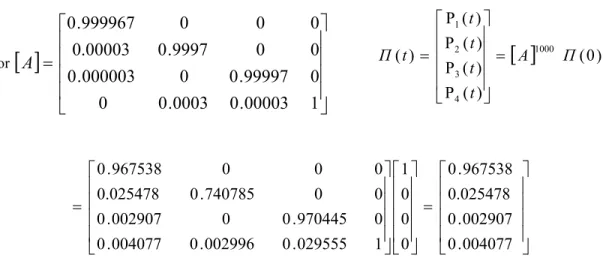
₍₃₂₎

If we divide the given mission time of 3 days into 1000 arbitrary time unit, then Δt = 3/1000 = 0.003 days. Substituting values of λ and Δt we have:

r12Δt = λ1Δt = 0.01(0.003) = 0.00003 r13Δt = λ2IΔt = 0.001(0.003) = 0.000003 r24Δt = λ2FΔt = 0.1(0.003) = 0.0003 r34Δt = λ1Δt = 0.01(0.003) = 0.00003 r11Δt = (λ1 +λ2I)Δt= 0.011(0.003) = 0.000033 r22Δt = λ2FΔt = 0.1(0.003) = 0.0003 r33Δt = λ1Δt = 0.01(0.003) = 0.00003 r44Δt = 0 Δt = 0

(14)

or

 















1

00003

.

0

0003

.

0

99997

.

0

000003

.

0

9997

.

0

0.00003

0

999967

.

0

A

 

(0) ) ( P ) ( P ) ( P ) ( P ) ( 1000 4 3 2 1 Π A t t t t t Π                                                     004077 . 0 002907 . 0 0.025478 967538 . 0 0 0 0 1 1 029555 . 0 002996 . 0 004077 . 0 0 970445 . 0 0 002907 . 0 0 0 740785 . 0 0.025478 0 0 0 967538 . 0

That is, the probability of being in state 1 (both generators operating) is P1(t) = 0.967538, the probability of being in

state 2 (generator X1 failed, X2 is operating) is P2(t) = 0.025478, the probability of being in state 3 (generator X2 failed while idle, X1 is operating) is P3(t) = 0.002907, and the probability of being in state 4 (both generators failed) is P4(t) = 0.004077.

4. Fault Tree Analysis

S1: System failure

S2: Station B unsupplied

S3: Station C

unsupplied supplied by a single line S4: Stations B and C

And

X1 S5: No supply

from C S6: No supply from B by cct 1 onlyS7: Supply

S8: Supply by cct 2 only

S9: Supply by cct 3 only

S10: CB

Tie out S11: CB Tie out

S12: AB Tie out And

And And And

X2 X3 X3 X3 X3 X2 X2 X2 X1 X1 X1 X4 X5 X4 X5 OR OR OR OR

(15)

Fault tree analysis is one of the most widely used technique for estimating system reliability and safety. Fault tree is a logic diagram that displays the interrelationships between a potential fault (accident) and its causes (Rausand, 2004). Causes may be due to environmental conditions, human errors, or a specific hardware/software failure. The basic operators used for building fault trees are AND (*) gates and OR (+) gates. An AND gate describes the logical operation that requires the coexistence of all input events to produce an output event. The OR gate describes that an output event occurs if any of the input events occur. Three basic types of events occur in a fault tree; 1) Top event, 2) Intermediate events, and 3) Terminal events. Typically, the undesirable event appears at the top of the fault tree and is placed within a rectangle. An intermediate event is any event within the fault tree that is further resolved into events that could cause it. These are represented by rectangles. A terminal or a sink event is an event that cannot be resolved into further causes and is represented by either circles or diamonds. The three event types are similar in concept to our notion of systems, sub-systems, and components. A power generator fault tree example adapted from (McCalley, 2005) is shown in Figure 12.

5. The Software Tool

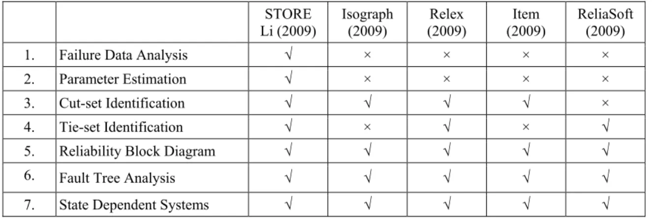
Currently, several software tools are required to conduct failure data analysis, parameter estimation, tie-set/cut-set identification, reliability block diagram analysis, analysis of state independent systems, analysis of state dependent systems, and fault tree analysis. Some of the tools are commercially available, while others are described in the literature by Semanderes (1971) – ReliaSoft (2009). This paper presents a revised Software Tool for Reliability Estimation (STORE) which was initially developed by Parekh (1999) and later revised by Li (2009). The revised tool, described here, not only integrates all of the above tasks, but is based on an efficient approach for representation and simplification of complex networks. The details of which were described by Ahluwalia (2011). The revised tool also utilizes a database to store and retrieve system, sub-system, and component data. The database enables users to build a library of sub-systems and components, which can be used to build new systems. The software was implemented in Microsoft Visual Basic 2008 with Microsoft SQL server as the database. It is not a commercial package, but can be obtained from the authors free of charge. A brief comparison of this software with the four (Isograph, Relex, Item, and ReliaSoft) commercial reliability software packages is provided in Table 12.

The software tool described above was applied to a variety of reliability problems described in open literature. The applications deal with component reliability estimation, estimation of reliability of state independent systems, estimation of reliability of state dependent systems, and fault tree analysis. The applications are intended to illustrate capabilities of the software from a practitioner’s point of view. The computational aspects of these tasks were described in sections 1-4. System simplification and enhanced computational efficiency are described in (Ahluwalia, 2011).

Table 12: Comparison of STORE with commercial software STORE Li (2009) Isograph (2009) Relex (2009) Item (2009) ReliaSoft (2009)

1. Failure Data Analysis √ × × × ×

2. Parameter Estimation √ × × × ×

3. Cut-set Identification √ √ √ √ ×

4. Tie-set Identification √ × √ × √

5. Reliability Block Diagram √ √ √ √ √

6. _{Fault Tree Analysis} _√ _√ _√ _√ _√

7. State Dependent Systems √ √ √ √ √

5.1 Component Reliability Estimation

Let’s say component X1 has a known reliability value of 0.93 and we wish to compute reliability of components X2-X6 from failure data. Let’s say failure data for component X2 was collected by testing fifteen units until they all failed (complete failure data). Time of each failure of component X2 is shown in Table 13. Twenty units of component X3 were

(16)

tested for 90 days (Type I single censored data). Time to failure of each unit is shown in Table 14. Fifty units of component X4 were tested till thirty five of them failed (Type II single censored). Failure times of component X4 are shown in Table 15. Fifteen units of component X5 were tested for 500 days. Failure times and censored (unit removed) times are shown in Table 16 (Type I multi censored data). A “+” next to the failure time indicates removal. Thirty units of component X6 were tested. Failure times are shown in Table 17 (Type II multi censored data). The data for these components was obtained from Ebeling (2005) in order to validate STORE. Screen shots of failure data analysis for components X2-X6 are shown in Figures 13-17, respectively. The “Analyze Distribution” button when clicked fits the four distributions (Exponential, Weibull, Normal, and Lognormal) to the failure data and displays distribution parameters. Results of the least squares method, MLE, and goodness-of-fit are also displayed for each distribution. The user can let the software pick the best distribution or select a distribution. The user can enter mission time of a given component and click “Calculate Reliability”. The reliability of the component is then displayed and saved in the database. The user can thus build a library of components with known distribution and reliability values, which can later be used to build a series, parallel, series-parallel, or a complex system.

Table 13: Complete failure data for component X2 Failure

Number 1 2 3 4 5 6 7 8 9 10 11 12 13 14 15

Time

(days) 25.1 73.9 75.5 88.5 95.5 112.2 113.6 138.5 139.8 150.3 151.9 156.8 164.5 218 403.1

(17)

Table 14: Type I single censored failure data for component X3 Unit

Number 1 2 3 4 5 6 7 8 9 10 11 12 13 14 15

Time

(days) 61.6 70 78.4 75.3 83.5 72.3 65.1 77.1 83.2 63.4 72.7 72.5 84.3 73 65.5

Figure 14: Analysis of Type I single censored data for component X3 Table 15: Type II single censored failure data for component X4

Failure Number 1 2 3 4 5 6 7 8 9 10 11 12 Time (days) 1.3 7.3 7.8 13.3 13.9 19.4 19.7 22.3 22.8 26.7 29.7 30.2 Failure Number 13 14 15 16 17 18 19 20 21 22 23 24 Time (days) 31.9 32.2 33 36.8 37 41.7 46.7 50.4 51.4 60 61.3 61.4 Failure Number 25 26 27 28 29 30 31 32 33 34 35 Time (days) 65.6 65.8 72.6 78.4 100.4 110.6 111.4 118.2 119.4 132.1 139.7

(18)

Figure 15: Analysis of Type II single censored data for component X4 Table 16: Type I multi censored failure data for component X5 Failure

Number 1 2 3 4 5 6 7 8 9 10 11

Time (days) 34 136 145+ 154 189 200+ 286 287 334 353 380+

Table 17: Type II multi censored failure data component X6 Failure Number 1 2 3 4 5 6 7 8 9 10 11 12 13 14 Time 141 391 399 410+ 463 465 497 501+ 559 563 579 580+ 586 616 Failure Number 15 16 17 18 19 20 Time 683 707 713 742+ 755+ 764

(19)

Figure 16: Analysis of Type I multi censored data for component X5

(20)

5.2 Reliability of State Independent Systems

Let’s say the six components (X1-X6) described above were organized to form a system as shown in Figure 18. The user can define the reliability block diagram of this system by entering component IDs under “Begin Node” and “End Node” and selecting the components from the database. The user can either assign reliability values to the components or use the values from the database. The software displays the system structure along with the reliability values of the system, sub-systems, and components. The software also displays all of the tie-sets associated with the system as shown in Figure 19.

Figure 18: Six component series-parallel system

Figure 19: Reliability of five component complex system

Nelson et al. (1970) analyzed a sixteen component complex system shown in Figure 20. They identified 55 tie-sets for this system. Figure 21 shows application of STORE to Nelson’s example. The various sub-system reliability values of the Nelson example are shown in Table 18. STORE's simplification algorithm when applied to this example reduced the

Start

X

2

X

3

X

4

End

X

1

(0.93)

X

5

X

6 1 2 3 4 5

(21)

number of tie-set from 55 to 1. The system when simplified turned out to be a simple series-parallel system and not a complex system as reported in (Ahluwalia, 2011).

Figure 20: Nelson's Example

Figure 21: Application of software to Nelson's example Start X1 (0.80) X2 (0.80) X3 (0.90) End X4 (0.85) X5 (0.75) X6 (0.82) X7 (0.82) X8 (0.89) X10 (0.85) X14 (0.75) X9 (0.88) X11 (0.85) X12 (0.85) X13 (0.80) X15 (0.70) X16 (0.70) 1 2 4 4 3 2 4 6 6 5 4 7 7 8 6

(22)

Table 18: Sub-system reliability values for the Nelson example Sub-system Reliability X1+X2 0.96 X3*X6 0.738 X4+X5 0.9625 X7+X8 0.9802 X15+X16 0.91 (X7+X8)*X9 0.862576 X11+X12+X13 0.9955 X14*(X15+X16) 0.6825 (X1+X2)*(X4+X5) 0.924 ((X7+X8)*X9)+X10 0.979386 ((X1+X2)*(X4+X5))+(X3*X6) 0.980088 (((X7+X8)*X9)+X10)*(X11+X12+X13) 0.974979 ((((X7+X8)*X9)+X10)*(X11+X12+X13))+(X14*(X15+X16)) 0.992056 (((X1+X2)*(X4+X5))+(X3*X6))*(((((X7+X8)*X9)+X10)*(X11+X12+X13)) +(X14*(X15+X16))) 0.972302

The STORE tool was also tested on other complex networks. These networks were reported by Gebre (2007), Fotuhi-Firuzabad et al. (2004), Ramirez-Marquez et al. (2006), and Lin et al. (2003). Table 19 shows number of cut-sets before and after application of simplification algorithm to the networks shown in Figure 22. The table also shows reduction of minimal cut-set for each network, in count and percent.

Table 19: Simplification of other complex networks

Network Source Minimal cut-sets before simplification Minimal cut-sets after simplification Reduction in minimal cut-sets (count) Reduction in minimal cut-sets (%) 1 Ramirez- Marquez (2006) 111 86 25 22.52% 2 Nelson (2007) 6441 4530 1911 29.67% 3 Nelson (2007) 330 214 116 35.15% 4 Nelson (2007) 615 191 424 68.94% 5 Nelson (2007) 888 250 638 71.85% 6 Nelson (2007) 222 23 199 89.64%

(23)

Figure 22: Other Complex Networks

5.3 Reliability of State Dependent Systems

Figure 23 shows the application of STORE to state dependent systems using the Markov model. The figure shows system reliability and each state’s reliability values for the two component standby system described in section 3.

2 3 4 5 6 11 1 7 8 9 10 12 1 4 2 5 1 8 9 3 6 7 10 11

2

2 1 3 4 6 5 7 8 10 9 11 12 14 13 15 16 3 2 3 4 5 6 7 8 10 11 18 12 1 13 14 17 9 16 15 4 2 3 5 6 17 9 8 4 10 11 7 14 13 15 16 12 1 5

(24)

Figure 23: Reliability of a state dependent system

5.4 Fault Trees

Figure 24 shows results of fault tree analysis for the system describe in Figure 12. STORE identified four minimal cut-set, {X3, X4, X5}, {X2, X3}, {X1, X3}, and {X1, X2}. If the unreliability values of components X1, X2, X3, X4, X5 were assumed to be R1′=0.1, R2′=0.2, R3′=0.3, R4′=0.4, R5′=0.5 respectively, then system survival probability (reliability) is equal to

(25)

Figure 24: Fault tree of a system from McCalley (2005)

6. Conclusions

This paper presented a software tool to computer reliability of components and sub-systems, and to store these values in a database. The component and sub-system data can be retrieved from the database to build new sub-systems and systems. A system can be a simple series-parallel system or a complex network. The software tool can identify failure distribution and associated parameters, for each component. It utilizes a novel approach to store and simplify complex networks. Components and sub-systems from the database can also be used to build and analyze fault trees.

The software tool was applied to various previously published case studies. In each case it identified either the same number or fewer tie-sets and cut-sets. The software tool is intended to introduce fundamental concepts of reliability to engineering student. Students should use the tool to verify hand calculations.

7. Reference

Ahluwalia, R. (2003), "A Software Tool for Reliability Estimation”, Journal of Quality Engineering, vol. 15, num., 4, pp 593-608.

Ahluwalia, R. S., Li, C, (2011). "An efficient approach to representation and simplification of complex networks", Computers & Industrial Engineering, vol. 61 pp. 525-523.

Ebeling, C. E. (2005). An Introduction to Reliability and Maintainability Engineering, Long Grove, IL, Waveland Press Inc. Fotuhi-Firuzabad, M., Billinton, R., Munian, T.S., Vinayagam, B. (2004), "A Novel Approach to Determine Minimal

(26)

Gebre, B. A., and Ramirez-Marquez, J. E., (2007), “Element substitution algorithm for general two-terminal network reliability analyses”, IIE Transactions, vol. 39, pp. 265-275.

Isograph, web site (2009). http://www.isograph-software.com/index.htm.

ITEM, web site (2009), ITEM software Inc., http://www.itemsoft.com/index.shtml.

Li, C. (2009), "Development of Software Tool for Reliability Estimation", MS Thesis, Industrial and Management Systems Engineering Department, West Virginia University

Lin, H.-Y., Kuo, S.-Y, and Yeh, F.-M., (2003). “Minimal cut-set enumeration and network reliability evaluation by recursive merge and BDD”, vol. 2, pp. 1341-6.

Magnier, M., Demick, B., and Williams, D., (2011), "Quake plunges Japan into fear, hardship", Los Angeles Times. McCalley, J. (2005). “Analysis of Non Series/Parallel Systems of Non-Repairable Components”, Power Learn Electric

Power Engineering Education, vol. module PE.PAS.U15.5.

Military Handbook (1990), Reliability Prediction of Electronic Equipment, MIL-HDBK-217F.

Nahman, J. M. (1994), "Enumeration of minimal paths of modified networks", Journal of Microelectronics and Reliability,

vol. 34, pp. 475-484.

Nelson A. C., Batts J. R., and Beadles R. L.(1970). “A Computer Program for Approximating. System Reliability”, IEEE Trans. Reliability, vol. R-19, pp. 61-65.

Pande, P. K., Spector, M. E. and Chatterjee, P., (1975), "Computerized Fault Tree Analysis: TREEL and MICSUP", Berkeley Operations Research Center, University. California of California, ORC-75-3.

Parekh, M., (1999), "Development of Decision Support System for Reliability", MS Thesis, Industrial and Management Systems Engineering Department, West Virginia University.

Ramirez-Marquez, J. E. and Coit, D. W., (2005), "A Monte-Carlo simulation approach for approximating multi-state two-terminal", Reliability Engineering and System Safety, vol. 87, pp. 253-264.

Ramirez-Marquez, J.E., Coit, D. and Tortorella, M., (2006). “A generalized multistate based path vector approach for multistate two-terminal reliability”. IIE Transactions, vol. 38, 6, pp. 477-488.

Rausand, M. and Høyland, A. (2004), System Reliability Theory: Models, Statistical Methods, and Applications. 2nd_edition. Hoboken, NJ, Wiley-Interscience.

Relex, web site (2009), Relex Software Corp., http://www.relex.com/ ReliaSoft, (2009), ReliaSoft Corp., http://www.reliasoft.com/.

Samad, M. A. (1978), "An efficient method for terminal and multi-terminal path set enumeration", Journal of Microelectronics and Reliability, vol. 27, pp. 443-446.

Schlager, N. (1994), When Technology Fails, Detroit Gale Group.

Semanderes, S. N. (1971), "ELRAFT: A computer program for the efficient logic reduction analysis of fault tree", IEEE Transactions On Nuclear Science, vols. NS-18.

(27)