SOLVING ECONOMIC DISPATCH PROBLEM USING PARTICLE SWARM OPTIMIZATION BY AN EVOLUTIONARY TECHNIQUE FOR INITIALIZING PARTICLES

(1)

665

AN EXTENDED STIPPLE LINE ALGORITHM AND ITS

CONVERGENCE ANALYSIS

ZHANDONG LIU∗∗∗∗_{, HAIJUN ZHANG, YONG LI, XIANGWEI QI, MUNINA YUSUFU}

Department of Computer Science and Technology, Xinjiang Normal University, NO. 102, New Medicine Road, Urumqi City, Xinjiang Province, China, 830054

ABSTRACT

Not only does the stipple line algorithm of previous have characteristics of a single type, but also the phenomenon, that the position of calculated pixel deviates from the actual line, appears easily when we solve practical problems. This paper introduces the previous stipple line algorithm. The other conditions of the stipple line algorithm are analyzed in detail. Last, the convergence of the stipple line algorithm is proved. The result shows that the vertical coordinate’s location, which the next pixel point of the current pixel point, converges weakly to the ideal line.

Keywords: Stipple Line Algorithm, Algorithm's Application, Convergence Analysis

1. INTRODUCTION

At present, the technology of computer graphics is widely used, and the research of computer graphics method is becoming more and more important. Curve drawing is the basic content of computer graphics, and the drawing of a straight line is based on the curve drawing [1].

In mathematics, the straight line, has no width, is a collection, which is composed of countless points. When the straight line is rasterized, we determine the best approximation to the straight line of a group of pixels, in which the display of the finite pixel matrix. According to the scan order, these pixels are operated by the current writing pattern. A picture may contain thousands of lines, so the speed of drawing algorithms must be as fast as possible.

The generating algorithm of classic line includes: Digital Differential Analysis (DDA) algorithm, stipple line algorithm and Bersenham algorithm[2]. DDA algorithm[3] need use the floating-point to calculate, so the accumulative error will make the calculated pixel position deviate from the actual line segment. Because the speed of pixel grid coordinate’s integer operations and floating-point calculations is very slow, the algorithm efficiency is very low, and DDA algorithm is rarely used in practice. The algorithms of stipple line and Bresenham overcome the disadvantages of DDA algorithm, are the most effective algorithm to create line. Literature [2], describes the stipple line algorithm, but its type is single. The phenomenon, that the position of calculated pixel deviates from

the actual line, appears easily when we use the algorithm which is introduced in the literature [2] to solve the practical problems. This paper introduces other situations of the stipple line algorithm, and analyses the convergence of the algorithm.

2. STIPPLE LINE ALGORITHM

2.1 Two Dimensional Line

In the plane coordinate, straight line can be expressed as ax+by+c=0.

For the straight segment whose starting coordinate is (xs, ys), the end coordinate is (xe, ye).

Its slope can be expressed as:

dx dy x x y y m

s e s

e =

− −

=( )₍ ₎

For any x, along the linear, whose increment is ∆x,

the increment of y is ∆y=m*∆x. For any ∆y,

m y x=∆ /

∆ .

∆x and ∆y constitute the foundations of

mathematics which determines the CRT(Cathode Ray Tube) deflection voltage. For the line segment which |m|≤1, firstly, we set the level component as ∆x. Then, according to the expression of

x m

y= ∆

∆ * , we can get the corresponding vertical

component of ∆y. For the line segment which |m|>1,

we set the vertical component as ∆y. Then,

according to the expression of ∆x=∆y/m, we can get the corresponding level component of ∆x. For

(2)

666 in the direction of coordinate where the adjacent pixels are taken[3-4].

2.2 Previous Stipple Line Algorithm

Let F(x, y) say the line segment of L(P0(x0, y0), P1(x1, y1)), the current pixel point is (xp, yp). For the

next pixel, there are two options to choose: P1(xp+1, yp) and P2(xp+1, yp+1). Let M(xp+1, yp+0.5) be the

midpoint of P1 and P2, Q is the crossing point of the

ideal line and x=x_p+1. We compare the position of Q and M. (a) When the point of M is located beneath the point of Q, P2 should be the next pixel; (b) When the point of Q is located beneath the point

of M, P1 should be the next pixel. As shown in

[image:2.612.138.267.272.357.2]

Figure 1.

Figure 1: Previous Stipple Line Algorithm

In order to judge the position relationship Q and

M, we need to put the M into the expression:

c

y)

F(x,

=

ax

+

by

+

. Then judge the symbols of

F(M)

. Now, we constructed discriminant:

c 0.5) b(y 1) a(x

0.5) y 1, F(x F(M) d

p p

+ + + + =

+ + = =

(1)

which

1

0 y

y a= − ,

0

1 x

x b= − ,

0 1 1 0y -x y

x

c=

_.

Because d is a line function of xp and yp, we use

incremental computing to improve the operational efficiency. Methods are as follows:

(a) When d≥0, we select the right point of P1 as

the next pixel. When the next pixel is determined, we calculate the expression:

a d+ =

+ + + + =

+ + + =

c 0.5) b(y 2) a(x

0.5) y 1, 1 F(x d1

p p

the increment is a.

(b) When d<0, we select the top right point of P2

as the next pixel. When the next pixel is determined, we calculate the expression:

b a d+ +

=

+ + + + =

c 1.5) b(y 2) a(x

1) 0.5 y 1, 1 F(x d2

p p

the increment is a+b.

Let’s begin to draw line from the point (x0, y0). By

Eq. 1, we know d0=a+0.5b. In order to eliminate

floating-point arithmetic, we use 2d to replace d. Algorithm program is shown as follows.

void Midpointline(int x0, int x1, int y0, int y1) {

dx=x1-x0; dy=y1-y0; x=x0, y=y0;

drawpixe1(x, y, color); if(dy/dx>0&&dy/dx<=1) {

d0=dx-2*dy; d1=-2*dy; d2=2*(dx-dy); while(x<x1) {

if(d0 >=0) x=x+1; d0=d0+d1; elseif(d0<0) x=x+1; y=y+1; d0=d0+d2;

drawpixe1(x, y, color) }

} }

2.3 Extended Stipple Line Algorithm

Let F(x, y) show the line segment of L(P0(x0, y0), P1(x1, y1)), the current pixel point is (xp, yp).

According to the slope size of the straight segment

L, for the next pixel point selection, we divide three

cases to analyse[5-9].

(1)When ₋₁_≤₋ _≤₀

b a

For the next pixel, there are two options to choose: P1(xp+1, yp) and P2(xp+1, yp-1). Let M(xp+1, yp-0.5) be the midpoint of P1 and P2, Q is the

crossing point of the ideal line and x=xp+1. We

compare the position of Q and M. (a) When the point of M is located beneath the point of Q, P2

should be the next pixel; (b) When the point of Q is located beneath the point of M, P1 should be the

(3)

667

P1

P=(xp,yp)

Q P2

P₁ M

Figure 2: The First Case Of The Stipple Line Algorithm

Now, we constructed discriminant:

c 0.5) b(y 1) a(x 0.5) y 1, F(x F(M) d p p p p + − + + = − + = = (2)

which a= y₀−y₁, b=x₁−x₀,

0 1 1 0y -x y

x

c= .

Because d is a line function of xp and yp, we use

(a) When d>0, we select the right-bottom point

of P1 as the next pixel. When the next pixel is

determined, we calculate the expression:

b a

d+ −

= + − + + = − + + = c 1.5) b(y 2) a(x 1) -0.5 y 1, 1 F(x d1 p p p p

the increment is a-b.

(b) When d≤0, we select the right point of P2 as

a d+ = + − + + = − + + = c 0.5) b(y 2) a(x 0.5) y 1, 1 F(x d2 p p p p

the increment is a.

Let’s begin to draw line from the point (x0, y0). By

Eq. 2, we know d0 =a−0.5b. In order to eliminate

floating-point arithmetic, we use 2d to replace d. Algorithm program is shown as follows.

dx=x1-x0; dy=y1-y0; x=x0, y=y0;

drawpixe1(x, y, color); if((dy/dx>=-1)&&(dy/dx<=0)) { d0=-dx-2*dy; d1=-2*(dx+dy); d2 =-2*dy; while(x<x1) {

if(d0 > 0) x=x+1; y=y-1; d0=d0+d1; elseif(d0<= 0) x=x+1; d0=d0+d2; drawpixe1(x, y, color); } } } (2) When

b

a

−

<

1

For the next pixel, there are two options to choose: P1(xp, yp+1) and P2(xp+1, yp+1). Let M(xp+0.5, yp+1) be the midpoint of P1 and P2, Q is

the crossing point of the ideal line and y=yp+1. We

compare the position of Q and M. (a) When the point of M is located left the point of Q, P2 should

be the next pixel; (b) When the point of Q is located right the point of M, P1 should be the next

[image:3.612.364.492.360.455.2]

pixel. As shown in Figure 3.

Figure 3: The Scond Case Of The Stipple Line Algorithm

c 1) b(y ) 5 . 0 a(x 1) y , 5 . 0 F(x F(M) d p p p p + + + + = + + = = (3)

which

a

=

y

₀

−

y

₁,

0

1 x

x b= − ,

0 1 1 0y -x y

x

c= .

Because d is a linear function of xp and yp, we use

(a) When d>0, we select the upper right point of P2 as the next pixel. When the next pixel is

b a d+ +

= + + + + = + + + + = c 2) b(y ) 5 . 1 a(x 1) 1 y 1, 5 . 0 F(x d1 p p p p

(4)

668

(b) When d≤0, we select the right above point of

P1 as the next pixel. When the next pixel is

b d+

=

+ + + + =

+ + +

=

c 2) b(y ) 5 . 0 a(x

1) 1 y , 5 . 0 F(x d2

p p

the increment is b.

Let’s begin to draw line from the point (x0, y0). By

Eq. 3, we know d₀ =0.5a+b. In order to eliminate floating-point arithmetic, we use 2d to replace d. Algorithm program is shown as follows.

dx=x1-x0; dy=y1-y0; x=x0, y=y0;

drawpixe1(x, y, color); if(dy/dx>1)

{

d0=2*dx-dy; d1=2*(dx-dy); d2=2*dx; while(y<y1) {

if(d0 >0) x=x+1; y=y+1; d0=d0+d1; elseif(d0<=0) y=y+1; d0=d0+d2;

drawpixe1(x, y, color); }

} }

(3)When ₋ _<₋₁

b a

For the next pixel, there are two options to choose: P1(xp, yp-1) and P2(xp+1, yp-1). Let M(xp+0.5, yp-1) be the midpoint of P1and P2, Q is

the crossing point of the ideal line and

y

=

y

p

+

1

. We compare the position of Q and M. (a) When the

point of M is located left the point of Q, P2 should

be the next pixel; (b) When the point of Q is

located right the point of M, P1 should be the next

pixel. As shown in Figure 4.

Figure 4: The Third Case Of The Stipple Line Algorithm

c 1) b(y ) 5 . 0 a(x

1) y , 5 . 0 F(x F(M) d

p p

+ − + + =

− +

= =

(4)

which

1

0 y

y

a= − ,

b

=

x

₁

−

x

₀,

c

=

x

₀

y

₁

-

x

₁

y

₀.

Because d is a linear function of xp and yp, we use

(a) When d>0, we select the below point of P1 as

b d−

=

+ − + + =

− +

=

c 2) b(y ) 5 . 0 a(x

2) y , 5 . 0 F(x d1

p p

the increment is -b.

(b) When d≤0, we select the right below point of

P2 as the next pixel. When the next pixel is

b a d+ −

=

+ − + + =

− + + =

c 2) b(y ) 5 . 1 a(x

2) y , 1 5 . 0 F(x d2

p p

the increment is a-b.

Let begin to draw line from the point of (x0, y0).

By Eq. 4, we know

d

0

=

0 .

5 a

−

b

. In order to

eliminate floating-point arithmetic, we use 2d to replace d. Algorithm program is shown as follows.

dx=x1-x0; dy=y1-y0; x=x0; y=y0;

drawpixe1(x, y, color); if(dy/dx<-1)

{

(5)

669 d2=-2*(dx+dy);

while(y>y1) {

if(d0>0) y=y-1; d0 =d0+d1; elseif(d0 <= 0) y=y-1; x=x+1; d0 =d0+d2;

drawpixe1(x, y, color); }

} }

3. THE APPLICATION OF EXTENDED

STIPPLE LINE ALGORITHM

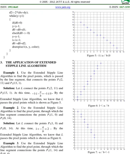
Example 1. Use the Extended Stipple Line

Algorithm to find the pixel points, which is passed by the line segment, that connects the points P1(2,

11) and P2(13, 1).

Solution: Let L connect the points P1(2, 11) and

P2(13, 1). At this time, −1≤− =−1≤0

b

a _{. By the}

Extended Stipple Line Algorithm, we know that L passes the pixel points which is shown as Figure 5.

Algorithm to find the pixel point, through which the line segment connections the points P1(1, 0) and P2(8, 14).

P2(8, 14). At this time, 1<− =2 b

a _{. By the}

Algorithm to find the pixel point, through which the line segment connections the points P1(1, 14) and P2(6, 4).

P2(6, 4). At this time, − =−2<−1

b

a _{. By the}

[image:5.612.89.522.58.573.2]

Figure 5: -1≤-a／b≤0

Figure 6: 1＜-a／b

Figure 7: -a／_b＜_-1

4. THE CONVERGENCE OF STIPPLE LINE

ALGORITHM

Definition: In the process of drawig line, let the

current pixel point be (xp, yp), and the vertical

coordinate be yk, horizontal coordinate be xk as the

next pixel position of (xp, yp). For any interval of [xp, xk], g(x) is a continuous function. When p>N, there

is

[

]

∫

− =

→ k p k

x

x k

x x

dx x g x f

y ( ) ( ) 0

(6)

670 where

k

and

p

is a natural number, in the

interval of [xp, xk], we say that {yk} weakly

converges to the function of f(x).

Theorem: In the interval [xp, xk], if the sequence

of {yk} converges to the function of f(x), and each yk

is continuous, then {yk} weakly converges to the

function of f(x).

Proof: In the interval of [xp, xk], let {yk}

converge to f(x), so f(x) is continuous. In the interval of [xp, xk], let g(x) be a continuous function.

By the probem set, in the interval of [xp, xk], we

know g(x).yk and g(x).f(x) are integrable[10-13]. In

the interval of [xp, xk], g(x) is continuous, so g(x)

has a maximal value, it is set to M(M>0). In the interval of [xp, xk], {yk} is uniform convergence to f(x). So for any positive number ε, there is N, when

P>N, for any x_∈[xp, xk], the expression:

M

x

f

y

p k k

)

(

)

(

−

<

−

ε

will be established. According to the properties of definite integral, when P>N, the expression_：

ε < −

≤

− =

−

∫

dx x f y M

dx x f y x g

dx x f x g dx y x g

k p k p k p

k p

x

x k x

x k

x x

x x k

) (

] ) ( )[ (

) ( ) ( )

(

will be established. So

∫

=

∫

→

k p

k p k

x x

x x k

x x

dx x g x f dx x g

y ( ) ( ) ( )

lim

.

That is to say {yk} weakly converges to f(x).

5. CONCLUSION

In this paper, the previous stipple line algorithm is introduced. Based on this, we expand the stipple line algorithm. Finally, we prove the convergence of the stipple line algorithm. The result showes that the stipple line algorithm has obvious weak convergence. The next step of the research is focused on the design of three dimensional midpoint algorithm, the efficiency of the algorithm and its application.

ACKNOWLEDGEMENTS

This work is supported by the University Scientific Research Project of Xinjiang Uyghur

Autonomous Region(XJEDU2012S29), the

Humanities and Social Science Project of China Ministry Education(11YJC870014), the National Nature Science Foundation of China (61163045), the National Nature Science Foundation of China (61263044), the Computer Application Technology Key Disciplines of Xinjiang Normal University.

REFERENCES:

[1] Q. F. Zhang, H. L. Wang, L. Zhang, ”Study on an algorithm of linear scan conversion”, Guizhou

University of Technoogy Journal, Vol. 32, No.

2, 2003, pp. 70-73.

[2] Andreas Löhne, Constantin Z˘alinescu, ”On convergence of closed convex sets”, Journal of

Mathematical Analysis and Applications, Vol.

319, 2005, pp. 617-634.

[3] Z. X. Wang, R. Y. Wang, ”Generalizing Midpoint Algorithm to 3D Straight-Line”,

Computer Simulation Journal, Vol. 24, No. 4,

2004, pp. 40-43.

[4] S. G. Zhao, H. X. Cao, ”Piontwise convergence of partial sums of wavelet expansions”, Pure

and Applied Mathematics Journal, Vol. 23, No.

1, 2007, pp. 113-119.

[5] Huaiyi Gao, Zhongdi Cen, ”The Convergence of a Midpoint Iterative Method with Milder Conditions”, Ning Xia University(Natural

Science Edition)Journal, Vol. 26, No. 1, 2005,

pp. 10-11.

[6] Zhandong Liu,Yugang Dai, ”An Improved Immune Algorithm and Its Convergence Analysis”, Proceedings of International Conference on Computer Design and Applications, IEEE Conference Publishing

Services, June 25-27, 2010, Vol. 1, pp. 164-166.

[7] Zhandong Liu, Tao Fu, Yugang Dai, Qinghua Zhao, ”A Study on the Convergence of the Clonal Select ion Algorithm Based on the Interval Sheath Theorem”, Journal of Computer

Engineering & Science, Vol. 32, No. 5, 2010,

pp. 57-59.

[8] Li Ma, Licheng Jiao, Lin Bai, ”Polyclonal Clusterring Algorithm and Its Convergence”,

China Universities of Posts and Telecommunications Journal, Vol. 15, No. 3,

2008, pp. 110-117.

[9] Juan A. Cljesta, Carlos Matran, ”Strong Convergence of Weighted Sums of Random Elements through the Equivalence of Sequences of Distributions”, Journal of Multivariate

(7)

671

[10] Xiaojun Chen, ”Superlinear convergence of

smoothing quasi-Newton methods for

nonsmooth equations”, Journal of

Computational and Applied Mathematics, 1997,

Vol. 80, No. 1, 1997, pp. 105-126.

[11] Moon-Soo Kim, Chulhyun Kim, ”On A Patent

Analysis Method for Technological

Convergence”, Journal of Procedia Social and

Behavioral Sciences, Vol. 40, 2012, pp.

657-663.

[12] Marek Balcerzak, Katarzyna Dems, Andrzej Komisarski, ”Statistical convergence and ideal convergence for sequences of functions”,

Journal of Mathematical Analysis and Applications, Vol. 328, No. 1, 2007, pp.

715-729.

[13] Jianping Luo, Xia Li, Mintong Chen, ”The Markov Model of Shuffled Frog Leaping Algorithm and Its Convergence Analysis”, Acta

Electronica Sinica Journal, Vol. 38, No. 12,