3809
A NEW MODEL FOR TRACKING AND DETECTION OF
DETERIORATION OF VITAL SIGNS BASED ON
ARTIFICIAL NEURAL NETWORK
¹TARIQ IBRAHIM ABDEL LATIF AL-SHWAHEEN, ²YUAN WEN HAU
UTM-IJN Cardiovascular Engineering Center, School of Biomedical Engineering and Health Sciences, Faculty of Engineering, Universiti Teknologi Malaysia, 81310 UTM Johor Bahru, Johor, Malaysia.
¹[email protected], ²[email protected]
Tracking and detection of the deterioration of vital signs has always been a challenging issue since it always happens suddenly and is associated firmly with serious problems such as recurrent readmissions of patients, increase the mortalities, and very little time window left for the clinician to take prompt medical action to treat the patient upon the detection. Many research have proposed various methods to predict and detect the deterioration of vital signs, but each of them has some strength and limitation, in terms of algorithm complexity and detection accuracy. This paper evaluates the capability of various Artificial Neural Network (ANN) models based on machine learning method to detect the deterioration of vital signs which consists of heart rate, blood pressure, body temperature and the saturation of oxygen in the blood. To evaluate and benchmark the detection accuracy of vital signs deterioration, various ANN models were constructed with the specific characteristics of each vital sign as input variables. Results show that the Levenberg-MarquardtANN model yields the highest detection accuracy of 95%, hence it is reliable in detecting the deterioration of vital signs.
Keywords: Artificial Intelligence (AI), Artificial Neural Network (ANN), Deterioration Of Vital Signs, Machine Learning, Prediction And Detection
I. INTRODUCTION
High Dependency Unit (HDU) or Intensive Care Unit (ICU) are hospital wards for the highly critical patients who need more intensive observation, treatment and nursing care. Their vital signs such as heart rate (HR), blood pressure (BP), body temperature (T) and saturation of oxygen in the blood (SPO2) are continuously monitored under close
observation. However, upon the detection of the critical state of one or more vital signs, normally there is not much time window left for the medical clinician to take prompt medical action to survive the patients. As a result, the delayed intervention of patients whose vital signs are deteriorating will likely increase morbidity and mortality [1]. Hence many active research have been conducted to seek an effective solution to address this problem, including machine learning approach.
The main principle of machine learning (ML) is deeply associated with computational statistics, which percepts a computer to detect, predict and learn principles using input data without being explicitly programmed. Thus, its primary goal is examining the solvable problems of a workable nature. Many
researchers nowadays agree that there is no intelligence without learning. In fact, some features are supposed to be compulsory in machine learning modeling, especially in treating the inputs with outliers and missing data. As a result, these features are helpful in solving medical issues to decrease the number of tests that are necessary to get a definitive diagnosis [1-4].
3810 Based on the aforementioned problems, this paper explores various Artificial Neural Network (ANN) algorithms, such as the Variable Learning Rate Backpropagation model, Bayesian Regularization model, Levenburg-Marquardt model and others, to compare and benchmark their accuracy performance in detection of the deterioration of many vital sign parameters. In this study, the targeted vital sign parameters consist of heart rate, blood pressure, body temperature and saturation of oxygen in the blood. The primary goal of this study was to investigate the possibility to track the deterioration of ICU’s or HDU’s patient based on these selected vital sign parameters using various ANN models to obtain good accuracy result.
This article is organized to six main sections. It begins with the introduction of machine learning and discussions of its issues and challenges in detecting deterioration of vital signs. Section II presents the critical review of related work. Section III presents the methodology from dataset collection until ANN architecture modelling. Section IV discusses the performance criteria, followed by Section V to discuss the result analysis. Section VI concludes the findings of this study and recommendations for future study.
2. RELATEDWORKS
There are many active studies investigate various algorithms in the detection of deteriorations of various vital signs, mainly in ML and deep learning (DL) methods. Chen et al. proposed the Random
Classification Model to predict the cardiorespiratory insufficiency based on heart rate (HR), respiratory rate (RR), saturation of oxygen in the blood (SPO2),
systolic blood pressure (SBP) and diastolic blood pressure (DBP), as the input vital sign variables [7]. The proposed monitoring systems have demonstrated usefulness in the dynamic distribution of technological and clinical personnel resources in critical care hospitals. They focus on the comparison of risk trends between the first four hours after step-down unit admission and the next four hours that happened immediately before the chronic renal insufficiency. However, this study is concluded based on the data obtained from a hospital of mostly postsurgical and trauma patients, hence it requires further research to generate a fully operational predictive model for a strict and potential framework.
Another work proposed by Lie et al. applied the
Couple Hidden Markov Model to predict the onset of septic shock based on input vital sign parameters of HR, RR and mean arterial pressure (MAP) [8]. The study reconstructed a patient instance as an ordered sequence of contrast patterns. The time-to-event prediction models are associated with Coupled Hidden Markov model and the results are compared against single variable Hidden Markov and Super Vector Machine models. The area under the receiver operating curve (AUC) trend given by the model was an aggregated measure of discernment through the hours prior to cardiorespiratory insufficiency events that is mainly driven by the diverse risk evolution types of the study patients.
Ordonez et al. proposed the K-Nearest Neighbor
model to predict a hypotension scenario based on input vital sign variables (SPO₂, SBP and DBP) within an hour [9]. This work applied their previous model as the baseline reference to benchmark their latest prediction performance in metrics of accuracy and precision. They proposed an algorithm to predict patient outcomes in ICUs that utilized likelihoods of edit distance costs. Time series data were modified to sequence performance to be utilized as inputs to algorithm. Various experiments were improved by altering the parameters through the conversion process. This study requires some parallel effort to strengthen the sequence length and hence further enhance the efficiency, as well as inspire a multivariate representation of the algorithm.
Another model proposed by Desautels et al.
applied the Continuous Nonlinear Function approximation to predict the sepsis onset based on input parameters of SBP, pulse pressure (PP), HR, RR, temperature, SPO₂, age and Glasgow Coma Scale (GCS) retrieved from electronic health records [10]. Despite using more parameters instead of only vital signs, the proposed model is considered an effective tool to predict sepsis onset and robust even with randomly missing data. However, this study does not include a collection of rules which imply a manual scoring system.
Lee et al. proposed an ANN model to predict the
3811 with each set consisted of 52 patients. The proposed algorithm demonstrated its performance by acquiring a sensitivity of 0.88, a specificity of 0.82, and an area under the receiver operating curve of 0.93. The main restriction of this study is data insufficiency, which gathered the data from 15 patient monitors within two years that have limited cases of ventricular tachycardia. This restriction limits the statistical power of the research's analysis. The authors also proposed another ANN model to predict the hypotensive events using vital signs of HR, SBP, DBP and Mean Blood Pressure (MBP) as input variables [12]. In addition, another ANN model is proposed to predict the hypotensive events with different variables which consist of MAP, HR, PP and relative cardiac output (CO) as the input vital signs. The promising pattern recognition performance has proven the presence of preferential patterns in hemodynamic data that can indicate impending hypotension. Moreover, a hypotensive risk stratified technique based on the pattern prediction algorithms proposed by the work could contribute clinical value in busy ICU environments [13].
Another model suggested by Ong et al. applied the
support vector machine (SVM) technique to predict the cardiac arrest based on many variables such as HRV, age, sex, medical history, HR, BP, SPO₂, RR and GCS within 72 hours [14]. Due to this study was performed at a tertiary hospital, it has limitation in term of generalization. In addition to that, whilst the machine learning score has been developed for internal validity, there is a necessity for external validation of the score for routine clinical utilization. The SVM algorithm is also adapted by Tang et al. to
predict the discrimination of severe sepsis from Systemic Inflammatory Response Syndrome patients based on electrocardiograph (ECG) signal and the Peak Pressure Gradient wave [15]. The data volume used in this work were just from 28 consecutive eligible patients attending the emergency department with presumptive diagnoses of sepsis syndrome. The classification results suggested that the combinatory use of cardiovascular spectrum analysis and the proposed SVM model of autonomic neural activity is a potentially useful clinical technique to classify the sepsis continuum into two separated pathological patterns of varying sepsis severity.
Crum et al. proposed the Bayesian Network Model
to predict the setting alerts from personal baselines [16]. The input variables consist of sex, age, temperature, HR, SPO₂ and admission diagnosis. The
Bayesian models were trained in machine learning, in combination with rule-based time-series statistical series are examined for the purpose of improving the accuracy of patient monitoring. The data used to train a set of the Bayesian net model were captured retrospectively from 36 patients admitted in ICU. Models were validated on a reserved dataset from another 16 additional patients based on the calculation of receiver operating characteristic (ROC) curves. The authors claimed that their techniques will improve the monitoring of ICU patients with high-sensitivity alerts, fewer false alarms, and earlier intervention.
Eshelman et al. developed a novel Repeated
Incremental Pruning to Produce Error Reduction (RIPPER) model to identify ICU patients that are likely to become hemodynamically unstable [17][2]. The rules of this model were created using a machine learning technique and were tested on retrospective data in the MIMIC II ICU database. The implementation model was not fully optimized, where it requires reconfiguration and fine-tuning when apply to other ICUs.
As concluding remark of literature review, it could be discovered that most algorithms target to specific datasets of patients with dedicated diseases. As a result, this proposed study investigates the possibility of tracking and detect the deterioration of patients with good accuracy, particularly patients at ICU and HDU, by relying solely on vital sign as input parameter, while filling the research gaps in the aforementioned related literature works, especially in terms of generalization in machines learning instead of targeted to specific disease.
3. METHODOLOGY
During the algorithm exploration in building various ANN models, many activities were involved such as dataset collection, identification of input vital sign variables and the number of outputs, as well as data processing steps. The detail of each activity is discussed in detail in the following subsections.
a. Dataset Collection
3812 clinical decision support and monitoring algorithms. It provides universal clinical data acquired from hospital medical information frameworks for tens of thousands of patients [18, 19].
This free database Physiological data of MIMIC II was obtained from patient monitoring devices which acquire and digitize multi-parameter physiological data. The monitoring devices also processed the signals to derive time series of clinical measurements such as HR, BP, and SPO₂. The data was then transmitted to a nursing central station network. The physiological signals (e.g. HR, BP, RR) were sampled at a frequency of 125 Hz.
In the proposed model, the clinical database was carefully selected to display the variations in vital signs readings. In this work, 14 datasets were extracted to hold as many various data as required. Each dataset contains about 600 readings that consist of five input vital signs, as listed below:
1. Systolic Blood Pressure (SBP) (in mmHg).
2. Diastolic Blood Pressure (DBP) (in mmHg).
3. Body Temperature (T) (in Celsius). 4. Heart Rate (HR) (in beats per minute). 5. Saturation of oxygen in the blood (SPO₂)
(as a percentage of 100%).
Every input is tabulated in a separate column in an Excel sheet, which leads to a total representation consists of five different columns. When applying
these data to MATLAB software, the readings of the columns will transpose into a raw data form. The graph plotting of the dataset readings is done by performing the following command in MATLAB:
DB1=xlsread(‘Database1.xlsx’);
(1.1)
plot(1:size(DB1,1),DB1(:,1)); (1.2)
b. National Early Warning Score (NEWS)
System
The NEWS system is based on a straightforward aggregate scoring system in which each physiological reading is assigned to a particular score [20]. The NEWS system was used during the algorithm exploration to validate the ANN computation output in MATLAB environment. There are four outputs, which are:
1. The output of SBP (MIMIC II deals mainly with the output of SBP and ignores the output of DBP).
2. The output of T. 3. The output of HR. 4. The output of SPO₂.
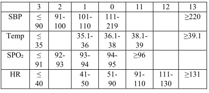
Depending on the NEWS system, each reading will have one output of the seven scores (3, 2, 1, 0, 1, 2, 3). However, MATLAB will not differentiate between the numbers to the right of the zero and the numbers which are on its left since they are identical. As a result, the numbers to the right of the zero were changed to the following values:
1 → 11, 2 → 12 and 3 →13.
[image:4.612.308.524.332.428.2]Table 1 shows the score values modifications:
Table 1: Revised NEWS System
3 2 1 0 11 12 13 SBP ≤
90 91-100
101-110
111-219
≥220
Temp ≤ 35
35.1-36
36.1-38
38.1-39
≥39.1
SPO₂ ≤ 91
92-93
93-94
94-95
≥96
HR ≤ 40
41-50
51-90
91-110
111-130
≥131
c. Data Pre-processing
The authors believe that networks trained with processed data can achieve better results than that trained with unprocessed data, due to the reason that processed data are subject to some cleaning and transformation steps to modify the raw data into a format that can be analyzed and visualized easily. NULL data is usually presented to compensate for missing or unknown values. It is extracted from the dataset to keep the flow of the information smooth. Other values that are extracted from the dataset are the NANs (Not A Number) values which represent undefined or unpresentable values.
3813 values. In this method, the dataset is visualized, then the outliers are identified by hand. After that, the outliers’ candidates are filtered out from the training dataset, and finally, assessing the model performance. Since the outliers in this model are identified for each feature independently, then, this type of outliers is considered as a univariate kind. Moreover, detecting the outliers is of significant importance since the dataset associated with this model is considered a quantitative discipline [22] [23].
It is well established that the original MIMIC II dataset is very large, so it is necessary to choose the right volume of data. The optimum volume of the dataset would be the minimum database that can perform the same duty without any loss of the performance. This step is called the instance selection step, where it is a strategy that deals with a trade-off technique between the reduction rate of the dataset and the classification quality. [24] [25].
The last step in the pre-processing phase is the normalization, which is a process of calculating the mean of each vital sign as well as reducing the data redundancy and improving the data integrity.
d. Feature Selection and Extraction
Sometimes, a lot of information may decrease the effectiveness of data mining [26]. So that, some of the columns assembled for performing and testing the model may not participate in implementing the model effectively. Some may indeed detract from the quality as well as the accuracy of the model [27]. Irrelevant attributes add noise to the data and may affect model accuracy. Noise increases the size of the model and the time needed to build it.
Each Excel Sheet consists of nine columns and about 600 rows, a target value of (1, 2, 3, 0, 11, 12, 13) has been assigned to the columns from six to nine. These target values represent the outputs of the vital signs referring to the NEWS system. In feature selection step, selecting the most relevant attributes is the target. Indeed, the vital signs that were selected are heart rate, blood pressure, saturation of oxygen in the blood and body temperature represent the selected features [28].
Indeed, feature extraction step transforms the attributes of the values. The transformed attributes, or features, are linear combinations of the main attributes. The target values indeed represent the extracted features. Then, the features become more significant to the classification process to obtain a higher accuracy level of prediction.
e. ANN Architecture Modeling
Building the architecture of the ANN model means determining the number of each type of the layers (input, hidden, output) as well as the number of nodes associated with these layers. Each neural network should have just one input layer. The number of nodes involved in this layer is the same as the number of the vital signs included in the dataset, which are HR, SBP, DBP, T, and SPO₂. As a result, the proposed model would have five nodes in the input layer [29] [30].
Likewise, every neural network has precisely one output layer without any exception. The number of outputs associated with the dataset determined the number of nodes involved in the output layer. As a result, each vital sign will be assigned to one out of the seven scores of the NEWS, which means there will be four nodes in the output layer, keeping in mind that DBP and SBP assigned to one target [31].
It is very imperative to mention that the hidden layer is the reason for naming the deep learning in this name. Since there is only one layer for both the input layer and the output layer for building most of the ANN models. Hence, determining the number of hidden layers and its underlying nodes is the most significant step in modeling. In fact, the cases and events in which the performance of the ANN model progresses in building more than one hidden layer seem rare. i.e., one hidden layer in building the ANN model is more than enough for most of the problems [17]. As a result, the proposed model also introduces one hidden layer. The hidden layer consists of a series of nodes that determine its size, and it can be examined as a consecutive (nonlinear) transformation of the input.
In the ANN model, the dataset is divided into three categories of training, validation and test dataset. The primary purpose of this division is to overcome the problems of overfitting and underfitting. Different algorithms were being used to build a novel model that gives a higher accuracy level. Finally, the Levenberg-Marquardt Training Model
(trainlm) is selected as the one with the most efficient
results. The trainlm algorithm is a numeric
minimization algorithm with an iterative procedure. It updates weight and bias values depending on Levenburg-Marquardt optimization. Researchers always considered trainlm as the fastest
3814 algorithm [32]. Moreover, this trainlm model
consists of one input layer of 5 nodes, one output layer of 4 nodes, and finally, one hidden layer of 50 nodes as shown in figure 1 below:
Figure 1: Structure of the proposed ANN Model
One of the important settings in building the ANN model is the number of the training iterations that is a recurring process to create a series of outcomes, with the purpose of approaching the desired goal. In the same way, a neural network is an algorithm that has the essential feature where it is performing training iteratively on the same data as well as on new data, hence, reducing the error with every single iteration. Training iteration would include the following steps:
1. Determining the cost function (a mechanism that returns the error between the targets and the outputs).
2. Modification of all weighting factors carefully.
Since the dataset is some appropriate thousands of values, it is divided into batches. When the whole dataset is being passed forward and backward through the neural network for just one time, this is called an Epoch. As the Epoch is too big and bulky to use on a computer as a whole dataset, it has been divided into batches [33].
The values of the initial weights and biases are chosen randomly so that the training algorithms might be applied twice with the same number of epochs and nodes and obtaining two different results. This happens because the initial values of the weights and biases are not the same at the beginning of the training. As a result, in MATLAB software, the weights and biases can be stored to save time.
After setting the values of the weights, the neural network can be trained to execute the specified function [34]. Generally, three datasets are required at different stages of ANN modeling, which are training dataset, validation dataset and test dataset. In the training dataset, the epochs are reiterated until the required output accuracy is obtained. The process of
determining the degree to which the model coincide to the real system, or at least precisely represents the model specifications and characteristics are referred to as model validation [35] [36].
4. PERFORMANCE CRITERIA
It is very crucial to evaluate an algorithm by considering its performance. In general, the R² value is considered the most universal statistical goodness-of-fit criteria to satisfy the performance of a classification model and it is known as the coefficient of determination. R² is widely used as a statistic value that is used in the cases of statistical models whose fundamental objective is the prediction of future outcomes. When the R² value is very close to 1, it means that there is an exact linear relationship between the outputs and the targets. The R² value reveals how well a model generates the predicted outcomes.
In this paper, the authors consider R² as a measurand of how the model replicated the observed findings [23] [24] [25]. Equation (1) below shows the calculations of R² value [37].
𝑅² ⅀ᵢ‗₁ ᵢ⅀ᵢ‗₁ ᵢ¯ ²⅀ᵢ‗₁ ^ᵢ¯ ^ᵢ ᵡ ²ᵡ ² (1)
where:
yᵢ: the experimental strength of the ᵢth specimen yˉ: the averaged experimental strength
y^ᵢ: the calculated compressive strength of the ᵢth specimen
y˟: the averaged calculated compressive specimen
5. RESULTS AND DISCUSSION
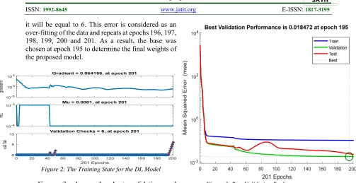
Figures 2 to 5 show the result graphs generated by MATLAB Simulink. Figure 2 shows the training state result of the proposed ANN model. The gradient demonstrates the slope of the tangent of the graph of the function. More precisely, the gradient points in the direction of the highest rate of increment of the function and its magnitude is the slope of the graph in that direction [38].
3815 it will be equal to 6. This error is considered as an over-fitting of the data and repeats at epochs 196, 197, 198, 199, 200 and 201. As a result, the base was chosen at epoch 195 to determine the final weights of the proposed model.
Figure 2: The Training State for the DL Model Figure 3 shows the best validation and performance based on the Mean Square Error value. The best validation performance is starting from a substantial Mean Square Error value that is more than 1000 and decreases to a minimal value of 195. The training line represents the training process of the training vectors that continue to decrease until the model reaches to a point that the training reduces the error of the network on the validation vectors, hence avoiding the over-fitting of the data sets. The primary purpose of the validation checks is ensuring that data have undergone data cleansing to ensure they have data quality, that is, that they are correct as well as useful. It implies routines, often called "validation rules" "validation constraints" or "check routines," that check for rightness, meaningfulness, and security of data that are input to the system [39]. It is shown that the best validation performance has happened at epoch 195 with a value of 0.018472.
[image:7.612.54.557.65.324.2]
Figure 3: Best Validation Performance
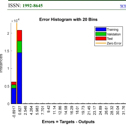
Figure 4 shows the error histogram with 20 bins (bars) for the whole training, validation and test steps in the proposed ANN modeling. The zero error is presented with a yellow line in the middle with 195 instances in the training set. The Y-axis represents the instances while the X-axis represents the errors. Bins are the number of vertical bars that can be observed on the graph. The total error from neural network ranges from -0.8917 (leftmost bin) to 2.5457 (rightmost bin). This error range is divided into 20 smaller bins, so each bin has a width of (2.5457 – (-0.8917)) / 20 = 0.1718.
3816 Figure 4: Error Histogram with 20 Bars for the Training,
Validation and Test Steps
Figure 5 clarifies the matching between the target and the output variables for training, validation, test and overall steps, respectively. The “Target” values imply “The Ready-Made Output of Vital Signs from the MIMIC II Dataset" and the “Output” values imply the “Predicted Outputs of Vital Signs by proposed ANN model. The R² value is calculated in MATLAB and represents the model performance efficiency. The figure illustrates that the R² values are equal to 0.94817, 0.98997, 0.98656 and 0.95945 for training, validation, test, and overall respectively.
Figure 5: Training, Validation, Test and Overall Results The nonlinear relation between the input variables (SBP, DBP, T, HR, and SPO₂) might be the main reason behind the efficiency of the model. Therefore, the DL can be considered as a reliable method for predicting and detecting the deterioration of the vital signs.
Different algorithms were used to implement a novel model that give the one with the highest accuracy. As well as various number of neurons in the hidden layer was selected such as 20, 30 and 50. Also, a different number of epochs were used such as 1000, 2000, 2500 and 3000.
It is very difficult to know the training algorithm with the fastest behavior and the highest accuracy for a given problem. There are many factors associated with these challenges such as the elaboration of the problem, the number of data points in the training set, the number of weights and biases in the whole network, the error target and whether the network is being used for pattern recognition (discriminant analysis) or function approximation (regression).
Table 2 illustrates the performance results of applying various algorithms in MATLAB. It is obvious that the trainlm is the one yield the best
results, the obtained accuracy performance was more than 0.98 and this number gives the worth to the training algorithm trainlm. In addition to the overall
R² value was approximately 0.96 which produce a good result.”
Table 2: The Results of Applying Various Training Algorithms in MATLAB
Training Algorithm
Description No of neurons
No of epochs
R² training
R² validation
R² test
R² overall
traingdx Variable Learning Rate Backpropagation
30 2000 0.34 0.38 0.34 0.35
trainbfg BFGS Quasi-Newton
30 2000 0.30 0.42 0.30 0.39
trainrp Resillient
Backpropagation 30 2000 0.70 0.59 0.53 0.65
traincgp Polak-Ribiere Conjugate
Gradient
30 2000 0.74 0.76 0.78 0.75
trainoss One Step Secant Backpropagation
30 2000 0.78 0.82 0.83 0.80
traincgf Fletcher-Powell
Conjugate Gradient
30 2000 0.80 0.82 0.85 0.81
trainbr Bayesian Regularization
30 2000 0.98 0.98 0.53 0.83
traincgb Conjugate Gradient with Powell/Beale restarts
30 2000 0.84 0.87 0.87 0.85
trainlm Levenburg-Marquardt
20 1000 0.94 0.98 0.98 0.95
trainlm Levenburg-Marquardt
30 2000 0.95 0.96 0.96 0.96
trainlm
Levenburg-Marquardt
30 3000 0.96 0.99 0.92 0.96
trainlm Levenburg-Marquardt
[image:8.612.325.587.427.708.2] [image:8.612.52.294.462.622.2]3817
6. CONCLUSION
This study has proven the deep learning algorithm is a reliable computational model to solve the problem of detecting and predicting the deteriorations of vital signs. It is due to the deep learning analysis implies a good correlation between the input variables and the output variables. Moreover, the statistical parameter R² for training, validation and testing steps denotes the real performance of the deep learning algorithm. As a result, the deep learning algorithm exhibits a good accuracy in predicting and detecting the deteriorations of vital signs. Therefore, instead of the continuous monitoring of the patients, the trainlm
model can be applied to perform this job more effectively and efficiently with best accuracy. As recommendations of future work, further study would explore other input variables such as lab tests and medical imaging scanning, to incorporate those parameters into machine learning modelling to further enhance the detection accuracy of deterioration of patients. In addition to that, a prediction model based on a considerable time window before the occurrence of deterioration of ICU’s patients will also be studied.
7. AKNOWLEDGEMENT
This research is supported and funded by Ministry of Higher Education (MoHE) Trans-Disciplinary Research Grant Scheme (TRGS) with Grant no. TRGS/1/2015/UTM/02/3/3 (UTM vote no. R. J130000.7845.4L842) and UTM International Doctoral Fellowship (IDF).
REFERENCES
[1]. 1. Kononenko, I., Machine learning for medical diagnosis: history, state of the art and
perspective. Artificial Intelligence in medicine,
2001. 23(1): p. 89-109.
[2]. 2. Kamio, T., T. Van, and K. Masamune, Use of Machine-Learning Approaches to Predict Clinical Deterioration in Critically Ill Patients:
A Systematic Review. International Journal of
Medical Research and Health Sciences, 2017.
6(6): p. 1-7.
[3]. 3. Zheng, T., et al., A machine learning-based framework to identify type 2 diabetes through
electronic health records. International journal of
medical informatics, 2017. 97: p. 120-127. [4]. 4. Bzdok, D. and A. Meyer-Lindenberg,
Machine learning for precision psychiatry. arXiv
preprint arXiv:1705.10553, 2017.
[5]. 5. Miotto, R., et al., Deep learning for healthcare: review, opportunities and
challenges. Briefings in bioinformatics, 2017.
[6]. 6. Lemley, J., S. Bazrafkan, and P. Corcoran,
Deep Learning for Consumer Devices and Services: Pushing the limits for machine learning, artificial intelligence, and computer
vision. IEEE Consumer Electronics Magazine,
2017. 6(2): p. 48-56.
[7]. 7. Chen, L., et al., Dynamic and Personalized Risk Forecast in Step-Down Units. Implications
for Monitoring Paradigms. Annals of the
American Thoracic Society, 2017. 14(3): p. 384-391.
[8]. 8. Ghosh, S., et al., Septic shock prediction for ICU patients via coupled HMM walking on
sequential contrast patterns. Journal of
biomedical informatics, 2017. 66: p. 19-31. [9]. 9. Ordoñez, P., et al., Learning stochastic
finite-state transducer to predict individual
patient outcomes. Health and technology, 2016.
6(3): p. 239-245.
[10]. 10. Desautels, T., et al., Prediction of sepsis in the intensive care unit with minimal electronic health record data: a machine
learning approach. JMIR medical informatics,
2016. 4(3).
[11]. 11. Lee, H., et al., Prediction of ventricular tachycardia one hour before occurrence using artificial neural networks.
Scientific Reports, 2016. 6: p. 32390.
[12]. 12. Lee, J. and R. Mark. A hypotensive episode predictor for intensive care based on
heart rate and blood pressure time series. in
Computing in Cardiology, 2010. 2010. IEEE.
[13]. 13. Lee, J. and R.G. Mark, An investigation of patterns in hemodynamic data indicative of impending hypotension in intensive
care. Biomedical engineering online, 2010. 9(1):
p. 62.
[14]. 14. Ong, M.E.H., et al., Prediction of cardiac arrest in critically ill patients presenting to the emergency department using a machine learning score incorporating heart rate variability compared with the modified early
warning score. Critical Care, 2012. 16(3): p.
R108.
[15]. 15. Tang, C.H., et al., Non-invasive classification of severe sepsis and systemic inflammatory response syndrome using a nonlinear support vector machine: a preliminary
study. Physiological measurement, 2010. 31(6):
p. 775.
3818
patient status in the intensive care unit. in AMIA
Annual Symposium Proceedings. 2009.
American Medical Informatics Association. [17]. 17. Eshelman, L.J., et al. Development
and evaluation of predictive alerts for
hemodynamic instability in ICU patients. in
AMIA Annual Symposium Proceedings. 2008.
American Medical Informatics Association. [18]. 18. Johnson, A.E., et al., MIMIC-III, a
freely accessible critical care database.
Scientific data, 2016. 3: p. 160035.
[19]. 19. Saeed, M., et al., Multiparameter Intelligent Monitoring in Intensive Care II (MIMIC-II): a public-access intensive care unit
database. Critical care medicine, 2011. 39(5): p.
952.
[20]. 20. McGinley, A. and R.M. Pearse, A national early warning score for acutely ill
patients. 2012, British Medical Journal
Publishing Group.
[21]. 21. Witten, I.H., et al., Data Mining:
Practical machine learning tools and techniques.
2016: Morgan Kaufmann.
[22]. 22. Rousseeuw, P.J. and A.M. Leroy,
Robust regression and outlier detection. Vol.
589. 2005: John wiley & sons.
[23]. 23. Garcia-Teodoro, P., et al.,
Anomaly-based network intrusion detection:
Techniques, systems and challenges. computers
& security, 2009. 28(1-2): p. 18-28.
[24]. 24. Song, Y., et al., An efficient instance selection algorithm for k nearest
neighbor regression. Neurocomputing, 2017.
251: p. 26-34.
[25]. 25. Arnaiz-González, Á., et al.,
Instance selection of linear complexity for big
data. Knowledge-Based Systems, 2016. 107: p.
83-95.
[26]. 26. Ratner, B., Statistical and machine-learning data mining: Techniques for better
predictive modeling and analysis of big data.
2017: Chapman and Hall/CRC.
[27]. 27. Micheli-Tzanakou, E., Supervised and unsupervised pattern recognition: feature
extraction and computational intelligence. 1999:
CRC Press.
[28]. 28. Novaković, J., Toward optimal feature selection using ranking methods and
classification algorithms. Yugoslav Journal of
Operations Research, 2016. 21(1).
[29]. 29. Bengio, Y., et al. Greedy layer-wise
training of deep networks. in Advances in neural
information processing systems. 2007.
[30]. 30. Mikolov, T., et al. Recurrent neural
network based language model. in Eleventh
Annual Conference of the International Speech
Communication Association. 2010.
[31]. 31. Samarasinghe, S., Neural networks for applied sciences and engineering: from
fundamentals to complex pattern recognition.
2016: CRC Press.
[32]. 32. Narang, A., et al., Classification of EEG signals for epileptic seizures using Levenberg-Marquardt algorithm based
Multilayer Perceptron Neural Network. Journal
of Intelligent & Fuzzy Systems, 2018. 34(3): p. 1669-1677.
[33]. 33. Escandell-Montero, P., et al.,
Online fitted policy iteration based on extreme
learning machines. Knowledge-Based Systems,
2016. 100: p. 200-211.
[34]. 34. Diab, A.M., et al., Prediction of concrete compressive strength due to long term
sulfate attack using neural network. Alexandria
Engineering Journal, 2014. 53(3): p. 627-642. [35]. 35. Khademi, F. and S.M. Jamal,
Predicting the 28 days compressive strength of
concrete using artificial neural network.
i-Manager's Journal on Civil Engineering, 2016.
6(2): p. 1.
[36]. 36. Crouse, M.S., R.D. Nowak, and R.G. Baraniuk, Wavelet-based statistical signal
processing using hidden Markov models. IEEE
Transactions on signal processing, 1998. 46(4): p. 886-902.
[37]. 37. Khademi, F., M. Akbari, and S.M. Jamal, Measuring compressive strength of puzzolan concrete by ultrasonic pulse velocity
method. i-Manager's Journal on Civil
Engineering, 2015. 5(3): p. 23.
[38]. 38. Lan, G. and Y. Zhou, An optimal randomized incremental gradient method.
Mathematical programming, 2017: p. 1-49. [39]. 39. Noetzelmann, O., et al., Method
and system for cross discipline data validation checking in a multidisciplinary engineering