2017 2nd International Conference on Computer, Mechatronics and Electronic Engineering (CMEE 2017) ISBN: 978-1-60595-532-2
Image Matching Based on ORB with Nonlinear Scale Space
Jun-hua YAN
1,*, Yong-qi XIAO
1, Zhi-gang WANG
1, Yin ZHANG
1,
Jing-cheng WANG
1and Sheng-xiang QI
21
College of Astronautics, Nanjing University of Aeronautics and Astronautics, Nanjing 210016, China
2
Science and Technology on Avionics Integration Laboratory, Shanghai 200233, China
*Corresponding author
Keywords: Image matching, Nonlinear scale space, ORB match, Scale invariance.
Abstract. To solve the problems of image precision loss and edge blur caused by SIRB (traditional improved ORB) algorithm when build multi-scale space using linear Gaussian pyramid, NORB (nonlinear scale space ORB) algorithm, which is based on the FED (Fast Explicit Diffusion) framework of nonlinear scale space structure, is proposed. Also, in order to overcome the limitation that after normalizing multi-scale space, there is a large number of repeatable (means multiple keypoints in the same image point) and unstable keypoints, the two-steps removing method is to put forward to filter the keypoints. Experimental results show that NORB exhibits scale invariance which is not possessed by the original ORB, effectively solves SIRB’s problem of accuracy loss, and manages to remove the unstable keypoints and repeatable keypoints, greatly improving the matching accuracy. Compared with the ORB and SIRB, although NORB slightly increases the time consumption, it obtains a higher matching accuracy and retains the high speed of the ORB algorithm at the same time, therefore overall, the detection efficiency is superior to other algorithms.
Introduction
Image matching, which is the technique of identifying effective keypoints for the matching between two images and calculating the coordinate transformation relations, is widely applied in fields such as image fusion, target tracking and motion detection [1-3]. SIFT [4-6] and SURF [7] are the most classical algorithms in image matching field, which construct the scale space by using the Gaussian. These two algorithms can both achieve relatively high matching accuracy, but have drawbacks of relatively low speed and accuracy loss due to the blurring of object boundaries caused by linear Gaussian kernel. The ORB[8] algorithm, which is put forward Ethan Rublee etc., has a matching speed higher than SIFT and SURF by two and one order of magnitude when the matching performance is similar, showing high real-time performance. Therefore it has a good application prospect. How to avoid the loss of accuracy in the process of constructing scale space [9], and retain a high real-time performance at the same time, is the key problem in image matching technology and its applications.
multi-scale space, we put forward ORB matching with nonlinear scale space [15] based on the FED framework; Also, in order to overcome the limitation that after normalizing multi-scale space, there is a large number of repeatable and unstable keypoints, the two-steps removing method is to put forward to filter the keypoints.
Related Works
This section gives a brief overview of the nonlinear diffusion filtering and fast explicit diffusion. Fast explicit diffusion framework is aimed to obtain low-computationally demanding features taking advantage of the benefits of nonlinear diffusion filtering.
Nonlinear Diffusion Filtering. Nonlinear diffusion filtering [16] sees the evolution of the luminance of an image through increasing scale levels as the divergence of a certain flow function, which can be described by nonlinear partial differential equations:
(
, ,)
L
div c x y t L t
∂
= ⋅ ∇
∂ (1)
where div and∇are the divergence and gradient operators respectively, L is the luminance of an image. c x y t
(
, ,)
is the conductivity function. By adjusting the conductivity function, it is possible to make the diffusion adaptive to the local image structure. t is the scale parameter. Larger values of t lead to simpler image representations. In anisotropic diffusion, the image gradient magnitude controls the diffusion at each scale level. Therefore, the conductivity function cis defined as:(
, ,)
(
(
, ,)
)
c x y z =g ∇Lσ x y t
(2) where the function ∇Lσ is the gradient of the Gaussian smoothed version of the original imageL. There are several conductivity functions that are possible to be used for g, but the conductivity function g2 promotes wide regions over smaller ones, which is used in AKAZE [17]:
2 2 2 1 1 g Lσ λ = ∇
+ (3)
where the parameter λ is the contrast factor that controls the level of diffusion. It determines which edges have to be enhanced or kept and which ones have to be deleted.
Fast Explicit Diffusion. FED schemes are inspired by a decomposition of box filters in terms of explicit schemes, in which iterated box filters approximate Gaussian kernels with good performance and are easy to accomplish [18]. The main idea of FED schemes is to divide explicit numerical iterative framework of diffusion equation into M outer cycles, and within each outer cycle, run n explicit diffusion steps with varying step sizes τj. The iteration time step is defined as:
max
2 2 1
2 cos ( )
4 2 j j n τ τ π = +
+ (4)
where τmax is the maximal step size that does not violate the stability condition of the explicit scheme. The corresponding stopping time within one FED cycle is obtained as:
2 1 max 0 3 n n j j n n
θ τ τ
−
=
+
=
∑
=the limitation of the explicit stability conditions. The discretization of Eq. (1) using an explicit scheme can be expressed in vector-matrix notation as:
1
( )
i i
i i
L L
A L L τ
+
− =
(6) where A L( )i is the image conductivity matrix, as the discretization version of conductivity
function. i
L is the luminance of an image in the i iterative, τ is a constant time step size, and max
τ<τ to meet the stability conditions. In explicit scheme, the solution i1
L+ is computed from the
solution at the previous evolution level i
L and image conductivities matrixA L( )i :
1 ( ( ))
i i i
L+ I τA L L
= + (7)
where I is the identity matrix. Considering the prior estimate i 1,0 i
L+ =L, a FED cycle with n variable step sizes τj is obtained as:
1, 1 ( ( )) 1, , 0... 1
i j i i j
j
L+ + I τ A L L+ j n
= + = −
(8) It is noteworthy here that the nonlinearities from the matrix A L( )i
are kept constant during the whole FED cycle. Once a FED cycle is done, we compute the new values of the matrixA L( )i . ORB with Nonlinear Scale Space
In this section we put forward a novel feature detection and description method. We use FED schemes for building a nonlinear scale space. To overcome the limitation that after normalizing the scale space, there is a large number of repeatable and unstable keypoints, the two-steps removing method is to put forward to filter the keypoints.
Building Nonlinear Scale Space. Traditional improved ORB algorithm uses linear Gaussian pyramid multi-scale decomposition to build scale space. However, this kind of linear decomposition will cause the loss of accuracy, blurring of the image edge, and loss of details. In order to solve this problem, we build ORB with nonlinear scale space based on the FED framework.
Similar to SIFT in the construction of the nonlinear scale space, scale level increases in accordance to the logarithmic. There are Ooctaves, each octave has S layers. Different octaves and layers are marked with serial numbers o and s respectively. The relationship between them and the scale parameter σ is shown in the equation below:
(
)
/[
]
, 2o s S, 0
i o s i M
σ +
= ∈ … (9)
whereo∈
[
0…O−1]
,s∈[
0…S−1]
, Mis the total number of images that go through the filter. Sincethe nonlinear diffusion filter is based on the scale of time, therefore scale parameters σi with the
unit of pixel is transformed to the unit of time as shown below:
[
]
2 1 , 0 2 i it = σ i∈ …M (10) where ti is called evolutionary time. For each input image, Gaussian filter is firstly applied, then
the gradient histogram of the image is calculated. The contrast factor λis set as 70% of the gradient histogram. In the case of 2D images, since the image derivative is a pixel grid size, the maximal step size tmax is 0.25 without violating stable conditions.
Given an input image 0
L , the contrast factorλ, the maximal step size τmax and a sequence of evolutionary timeti, all smoothed images can be acquired using nonlinear scale space based on the FED framework by the following steps:
Step2: Set one FED outer cycle timeT =ti+1−ti.
Step3: Compute the smallest number of FED inner steps n so that θ ≥n T, and define that
n q=T θ .
Step4: Compute iterative step sizesτj=τj⋅q. Step5: Set prior estimation Li+1,0 Li
= as the initial value of the inner loop.
Step6: According to the Eq. (8), compute the layer i+1 of the image through the calculation of inner cycle in the FED.
Step7: Ifoi+1>oi, then use the downsample image layer
1
i
L+ with smooth mask (0.25, 0.5, 0.25) as the starting image for the next FED cycle in the next octave. Recalculate the contrast factorλ λ= ⋅0.75.
Step8: If the outer loop indexi<M, then repeat the cycle again from step 1.
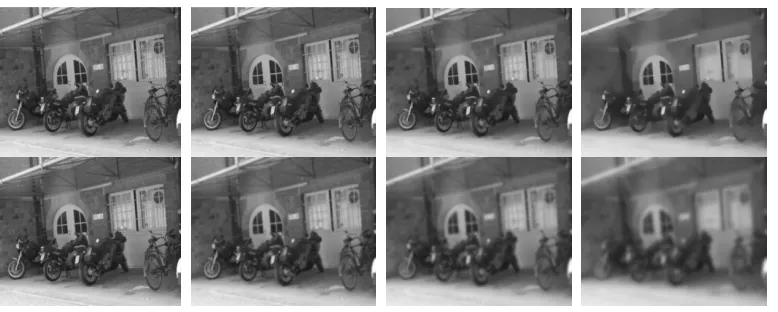
[image:4.612.115.504.241.397.2]The results of the nonlinear scale space built by following the above steps are shown in Fig.1:
Figure 1. Comparison between the nonlinear diffusion (first row) and Gaussian (second row) scale space for several evolution times.
The first row of Fig. 1 shows the results of building nonlinear scale space using nonlinear diffusion. The evolution increases gradually and the soothing degree becomes higher form left to right. The second row shows the results of constructing linear scale space by convolving the original image with a Gaussian kernel of increasing standard deviation. Similarly, the evolution increases gradually and the soothing degree becomes higher form left to right.) The evolution time of the nonlinear scale space and Gaussian scale space is the same in each column. As demonstrated clearly in Fig. 1, Gaussian filtering causes loss of precision, blurring of the image edge and loss of details, while nonlinear filtering can reserve details such as image edges.
Feature Detection. In traditional improved ORB algorithm, features are extracted by detecting the ORB keypoints of interest separately in each layer from the multi-scale pyramid images, maintaining a good scale invariance. However, when describing feature keypoints, features extracted from each layer need to be normalized to the original image space, resulting in a large number of repeatable keypoints and some uncertain keypoints, and thus reducing the accuracy of image matching.
delete repeated
points delete unstable
points
[image:5.612.202.413.67.174.2]Normalize scale space
Figure 2. Feature detection by using a two-step method.
Feature Description. Feature description is established based on the structure of the original ORB algorithm: randomly select several 5 5× pixel blocks in the adjacent field of the point with
31 31× pixels, compare the pixel blocks using integral image, calculate the binary string as the initial description of the keypoints. This method can effectively reduce the interference of random noise. To achieve rotation invariance, add direction information to BRIEF, use greedy search method at the same time. Extract the first 256 pairs of features with lowest correlation and finally acquire the feature descriptor rBRIEF of NORB.
Process of NORB Algorithm. Aiming at improving on the problems of traditional improving ORB method, which are precision loss of linear decomposition and the appearance of unstable and repeatable keypoints, we put forward NORB algorithm to improve the performance of matching and meanwhile ensure fast computation. Steps of NORB algorithm are as follows:
Step 1: Build nonlinear scale space using the FED structure.
Step 2: Eliminate repeatable and unstable keypoints to achieve the features with scale invariance. Step 3: Build NORB feature descriptor.
Step 4: Match the keypoints through comparing the hamming distance. Experimental Results
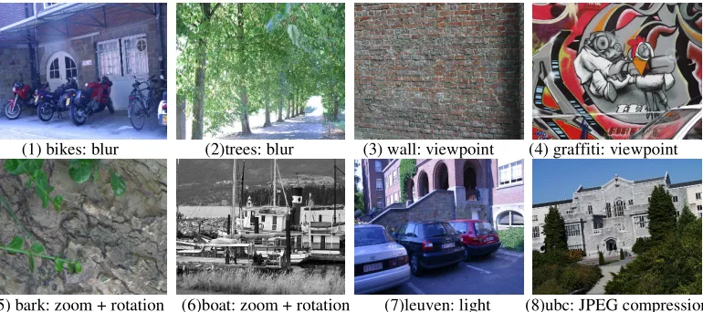
We use the standard dataset from Mikolajczyk[20] to evaluate the performance of detector, we compare NORB algorithm with original ORB and traditional SIRB algorithm. The dataset contains 8 groups, and each group contains six high resolution images with different geometric and photometric transformations such as image blur, lighting, viewpoint, zoom, rotation and JPEG compression, as shown in Fig. 3. In addition, the ground truth homographies are also available for every image transformation with respect to the first image of every sequence. Using the dataset is a good way to test the performance of feature detection algorithm. Experimental environment: Visio Studio 2013 + OpenCV3.0, equipment configuration: 2.00 GHz, dual processor, 32G installed memory. We also show in Fig. 4 an example of images with matched keypoints. The number of keypoints in both images is approximately the same, but with the proposed algorithm the number of matches is much higher.
(1) bikes: blur (2)trees: blur (3) wall: viewpoint (4) graffiti: viewpoint
[image:5.612.114.499.559.730.2]
(1)SIRB (2)NORB
Figure 4. Matches of ORB keypoints detected using different filters in a pair of images from ubc sequence. Green keypoints are the detected ones, and blue keypoints are matched.
Detection Precision Experiments. Precision [21] is defined as the ratio of the number of correct matching keypoints and that of matching keypoints. The larger the ratio is, the better the performance. Using various matching methods, the results of precision of different data sets with different geometric and photometric transformations such as blur and viewpoint are shown in Fig. 5. The experimental results show that the NORB algorithm has stronger adaptability for the datasets with blur, lighting, viewpoint, zoom, rotation and JPEG compression and the performance is better. Also, when the degree of transformation increases, the matching performance is reduced. As for the change of illumination, the precision of NORB algorithm and that of two other are similar, thus the performance is not enhanced.
Figure 5. Results of precision on different datasets.
Figure 6. Results of matching rate on different datasets.
Detection Time Experiments. Minimizing the time of the combined detection and description is crucial for the algorithm to be realized in real-time.) Using the same local feature detection algorithm, the numbers of extracted features for different images are different, and so is the time cost. Using different local feature detection algorithms, the numbers of extracted features for the same image are different, and so is the corresponding time cost. The NORB algorithm adopts the same way of feature detection and description as the ORB and SIRB, and compared with the ORB and SIRB, the main improvement of NORB algorithm is to build nonlinear scale space, and the costing time is listed. As shown in Table 1, the average is 63ms. The experimental results show that NORB algorithm obtains higher matching accuracy at the cost of a slightly increase in the time consumption.
Table 1. Costing time of building nonlinear scale space (ms).
frame bikes tress graf wall bark boat leuven ubc
1st 74 92 70 80 80 56 95 63
2nd 87 74 58 63 54 74 69 54
3rd 65 71 79 58 62 48 67 50
4th 68 72 77 63 62 49 85 52
5th 74 86 81 99 64 43 79 90
6th 79 70 56 66 56 57 65 46
Timing Evaluation. The comparison of the time cost of NORB matching algorithm and other feature detection and description algorithms is shown in Fig. 7. The experimental results show that compared with SIRB and ORB, although the total time consumption of NORB features detection algorithm increases, it exhibits the scale invariance which is not possessed by the original ORB and effectively solves SIRB’s problem of precision loss. Thus, the matching accuracy is significantly improved. NORB retained the high speed of the ORB algorithm, compared to SIFT and SURF algorithm, it has a better real-time performance. We also show in Fig. 8 an example of tracking deformable object with scale, location and rotation changing by using the proposed algorithm. The sequence’s size is 1224 1024× pixels. Because of temporal context, we set a search widow with
400 400× pixels, and achieve the tracking rate of 36fps.
Figure.8 Sequence of tracking object by using NORB.
Conclusion
To solve the problems that algorithm based on traditional improved SIRB spoils accuracy and to overcome the limitation that after normalizing the scale space, there is a large number of repeatable and unstable keypoints, we put forward NORB algorithm. The results of the experiment based on the datasets with different geometric and photometric transformations such as image blur, lighting, viewpoint, zoom, rotation and JPEG compression show that: NORB algorithm significantly improves the precision and matching rate except for under the condition of light changes, and at the same time, it retains the high speed of ORB algorithm. The main possible reason why the NORB did not improve the performance under the condition of light changes is that the construction of nonlinear scale space is sensitive to light. We will conducted further research in the future.
Acknowledgments
This work was supported by the National Natural Science Foundation of China (61471194, 61705104), Science and Technology on Avionics Integration Laboratory and Aeronautical Science Foundation of China (20155552050), China Scholarship Council Foundation (201506835020), the Natural Science Foundation of Jiangsu Province (BK20170804).
Conflict of Interest
The authors declare that they have no conflict of interest.
Reference
[1] Liu C, Yuen J, Torralba A: Dense scene alignment using SIFT flow for object recognition. IEEE Conf. on Computer Vision and Pattern Recognition, CVPR (2009).
[2] Je C, Park H M: Optimized hierarchical block matching for fast and accurate image registration. Signal Processing: Image Communication, 28(7): 779-791 (2013).
[3] Saha A, Mukherjee J, Sural S: A neighborhood elimination approach for block matching in motion estimation. Signal Processing: Image Communication, 26(8): 438-454 (2011).
[4] Lowe D G: Distinctive image features from scale-invariant keypoints. International journal of computer vision, 60(2): 91-110 (2004).
[5] Amin Sedaghat, Hamid Ebadi: Remote Sensing Image Matching Based on Adaptive Binning SIFT Descriptor. IEEE Transactions on Geoscience and Remote Sensing, 53(10): 5283-5293 (2015).
[7] Bay H, Tuytelaars T, Van Gool L: Surf: Speeded up robust features. Computer vision– ECCV 2006. Springer Berlin Heidelberg, 404-417 (2006).
[8] Rublee E, Rabaud V, Konolige K, et al: ORB: an efficient alternative to SIFT or SURF. IEEE International Conference on Computer Vision. Barcelona, Spain, 2564-2571 (2011).
[9] Wang S, You H, Fu K: BFSIFT: A novel method to find feature matches for SAR image registration. Geoscience and Remote Sensing Letters, IEEE, 9(4): 649-653 (2012).
[10] Xiao Bin, Jiang Yi, Lin Fan: Mobile Augmented Reality 3D Registration Algorithm Based on ORB and KLT. Computer and Modernization, 03: 57-60+64 (2014).
[11] Xu HK, Qin YY, Chen HR: Based on the improved ORB image feature point matching. Science Technology and Engineering, 18: 105- 109+ 128 (2014).
[12] Duits R, Florack L, De Graaf J, et al: On the axioms of scale space theory. Journal of Mathematical Imaging and Vision, 20(3): 267-298 (2004).
[13] Alcantarilla P F, Bartoli A, Davison A J: KAZE features. Computer Vision–ECCV 2012. Springer Berlin Heidelberg, 214-227 (2012).
[14] Weickert J, Romeny B H, Viergever M A: Efficient and reliable schemes for nonlinear diffusion filtering. Image Processing, IEEE Transactions on, 7(3): 398-410 (1998).
[15] S. Grewenig, J. Weickert, and A. Bruhn: From box filtering to fast explicit diffusion. In Proceedings of the DAGM Symposium on Pattern Recognition, (2010).
[16] Perona P, Malik J: Scale-space and edge detection using anisotropic diffusion. Pattern Analysis and Machine Intelligence, IEEE Transactions on, 12(7): 629-639 (1990).
[17] Alcantarilla P F, Solutions T V: Fast explicit diffusion for accelerated features in nonlinear scale spaces. IEEE Trans. Patt. Anal. Mach. Intell, 34(7): 1281-1298 (2011).
[18] Grewenig S, Weickert J, Schroers C, et al: Cyclic schemes for PDE-based image analysis. Dept. Math., Saarland Univ., Saarbrücken, Germany, Tech. Rep, 327 (2013).
[19] Harris C, Stephens M: A combined corner and edge detector. Alvey vision conference., 15: 50 (1988).
[20] Mikolajczyk, K., Tuytelaars, T., Schmid, C., et al: A comparison of affine region detectors. Intl. J. of Computer Vision 65, 43–72 (2005).
[21] Mikolajczyk, K., Schmid, C: A performance evaluation of local descriptors. IEEE Trans.Pattern Anal. Machine Intell. 27, 1615–1630 (2005).