Study of Existing Tall Building by Using Pushover Analysis

(1)

STUDY OF EXISTING TALL BUILDING BY USING PUSHOVER ANALYSIS

A. Amarnath

1

_{, Sajeet S.B}

2

_{,Tejaswini Betgeri}

3

1

Assistant Professor, Civil Engineering Dept. S.G. Balekundri Institute of Technology, Belagavi, Karnataka, India

₂

Structural Design Consultant, Bengaluru, Karnataka, India

3

M.Tech student of S.G.Balekundri Institute of Technology, Belagavi, Karnataka, India

---*---Abstract -**

This study deals with the assessment of seismic performance of an existing building using non linear static analysis or Pushover analysis. The selection of G+13 existing building was with an intension to serve for commercial purpose. Analysis was carried out using ETABS 9.7.1 and also analysis of the same existing tall building which has to serve for Industrial purpose is carried out. The structural model with typical storey height of 3.5m is developed and then seismic behavior of commercial as well as Industrial buildings having LL of 4kN/m2_{and 7kN/m}2_{respectively are studied} using Pushover analysis. By comparing the results one can identify whether retrofitting is recommended or not in this study.

Key Words:

Seismic performance, Pushover analysis,

Retrofitting.

1. INTRODUCTION

Structural engineering is having tremendous need with advancement of science and technology. One of the simple and noticeable methods is Pushover analysis which considers non linear characteristics of materials but deals with only static load cases. This analysis has become most preferred analysis method for seismic evaluation of buildings and design purposes as it is relatively simple and post elastic behavior is considered.

1.1 PUSHOVER ANALYSIS

It is a static non linear analysis under permanent vertical loads and gradually increasing lateral loads. It is a popular tool for seismic tool for seismic performance evaluation of existing and new structures. The necessity of Pushover analysis is that, as Indian buildings built over decades are seismically deficient due to lack of awareness regarding seismic behaviour of structures, it generates great demand for seismic evaluation and retrofitting of existing buildings.

Fig -1: Force-Deformation Relation in Pushover Analysis

1.2 OBJECTIVES

1. To determine the effective method to find strength of concrete over Non-Destructive Tests (NDT) on existing commercial building using Static Analysis.

2. The performance and behaviour of the existing commercial building is studied using pushover analysis. 3. To study the performance and behaviour of existing building which has to serve as Industrial building using pushover analysis.

4. To study behaviour of the retrofitted Industrial building by pushover Analysis.

2. STRUCURAL MODEL

Model is done using ETABS 9.7.1. The structural models story height of 3.5m is kept same and live load of 4kN/m2

for commercial building and 7kN/m2_{for Industrial}

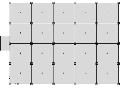
Building. Building plan is shown is figures below.

[image:1.595.351.516.232.300.2] [image:1.595.318.532.574.729.2]

(2)

Fig -3: T2 type of Industrial Building

Fig -4: T3 type of Retrofitted Industrial Building

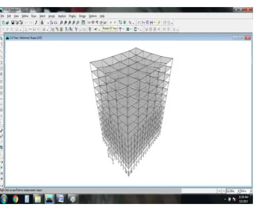
Fig -5: 3D view of T3 model after analysis

2.1 Types of models

There are three types of model

- Commercial building with live load of 4kN/m2 _(TYPE1)

-Industrial building with live load of 7kN/m2_(TYPE2)

- Retrofitted Industrial building with live load of 7kN/m2

[image:2.595.46.272.111.486.2]

(TYPE3)

Table -1: Section Details

COL BEAM SLAB

TYPE1 B-14 C 300X300 B 250X500 200

C 700X700 B 700x700 200

TYPE2 B-14 C 300X300 B 250X500 200

C 700X700 B 700x700 200

TYPE3 B-14 C 300X300 B 250X500 200

C 700X700 B 700x700 200

Dbl.ISMB550

Table -2: SEISMIC LOADING ZONE AS PER IS:1893 2002

DETAILS VALUE

R 5

I 1.5

Z 0.24

[image:2.595.58.269.112.284.2]

Sa/G Type2

Table -3: Material Properties MODEL TYPE

MATERIAL PROPERTIES All Model

Column M35

Beam M25

Slab M25

Slab thickness: 200mm

Dead Load: Floor finish = 2 kN/m2

Roof floor finish = 3 kN/m2

Imposed Load: On roof 1.5 kN/m2

Hinge Assignment Beams : default M3=0 default M3=1 Columns: default P-M-M =0

default P-M-M =1 Static non linear data for PUSH1 DL=Dead load factor 1

[image:2.595.51.566.139.747.2] [image:2.595.300.567.199.560.2] [image:2.595.37.293.521.724.2]

(3)

3. RESULT AND DISCUSSION

[image:3.595.323.542.62.374.2]

DETERMINATION OF GRADE OF CONCRETE

Table -4: Calculation of Compressive strength of concrete(fck)

Col size(mm) 700X700 (Characterstic

strength of

steel) fy 500 N/mm2

Rebar

percentage 2.93 %

(Axial load)

Pu= 10553 kN

(Area of

concrete)

Acon= 490000 mm2

(Area of steel)

Ast= 14357 mm2

(Area of

cement)Ac= 475643 mm2

(Compressive strength of

concrete)fck= 32.82871818 N/mm2

Therefore,fck= 35 N/mm2

3.1 Pushover Curves

Type1 model, the ultimate base shear is around 9307 kN and the corresponding roof displacement is 467mm is shown in Fig 6

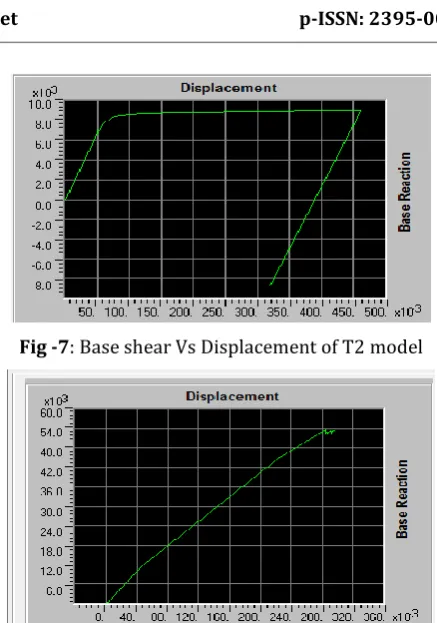
Type2 model, the ultimate base shear is around 9078kN and the corresponding roof displacement is 461mm is shown in Fig 7

Type3 model, the ultimate base shear is around 53640kN and the corresponding roof displacement is 297 mm is shown in Fig 8

Fig -6: Base shear Vs Displacement of T1 model

3.2 Capacity Spectrum

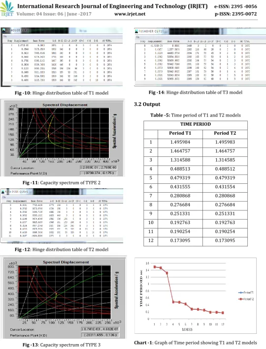
The base shear at performance point is 8824kN and corresponding displacement is 175mm is shown in Fig 9 overall performance of building is said to be Live safety to Collapse prevention.

The base shear at performance point is 8798kN and corresponding displacement is 175 mm is shown in Fig 11 overall performance of building is said to be Live safety to Collapse prevention.

The base shear at performance point is 28311kN and corresponding displacement is 136mm is shown in Fig 13. overall performance of building is said to be in Immediate occupancy.

[image:3.595.50.270.161.402.2] [image:3.595.50.276.167.403.2] [image:3.595.52.269.552.685.2] [image:3.595.326.543.592.732.2]

(4)

Fig -10: Hinge distribution table of T1 model

Fig -11: Capacity spectrum of TYPE 2

[image:4.595.36.577.43.754.2]

Fig -13: Capacity spectrum of TYPE 3

[image:4.595.328.542.291.590.2]

3.2 Output

Table -5: Time period of T1 and T2 models

TIME PERIOD

Period T1 Period T2

1 1.495984 1.495983

2 1.464757 1.464757

3 1.314588 1.314585

4 0.488513 0.488512

5 0.479319 0.479319

6 0.431555 0.431554

7 0.280868 0.280868

8 0.276684 0.276684

9 0.251331 0.251331

10 0.192763 0.192763

11 0.190254 0.190254

12 0.173095 0.173095

(5)

[image:5.595.315.556.54.242.2]

DISPLACEMENTS

UX T1 UX T2

13 422.2494 411.0996

12 420.9112 409.7873

11 417.273 406.6111

10 407.789 398.7492

9 388.4553 382.1157

8 356.8933 353.5165

7 312.7363 311.9642

6 257.6478 258.7104

5 194.5703 196.6772

4 130.3103 132.5415

3 72.8918 74.4512

2 28.631 29.3591

1 3.8301 3.9467

BASE 0 0

[image:5.595.39.283.114.514.2]

Chart -2: Graph of Displacement (mm) showing T1 and T2 models

Table -7: Storey Drift ratio of T1 and T2 models

STOREY DRIFTS

DriftX T1 DriftX T2

13 0.000729 0.000695

12 0.001606 0.00143

11 0.003482 0.002963

10 0.006471 0.005635

9 0.010106 0.009187

8 0.013804 0.012982

7 0.016947 0.01635

6 0.018951 0.018638

5 0.019324 0.019271

4 0.017715 0.01783

3 0.013982 0.014136

2 0.00822 0.008321

1 0.002367 0.002385

Chart -3: Graph of Storey Drift ratio showing T1 and T2 models

Table -8: Storey Shear of T1 and T2 models

STOREY SHEAR

VX T1 VX T2

13 -664.41 -714.63

12 -1266.15 -1361.86

11 -1768.38 -1902.05

10 -2180.08 -2344.88

9 -2510.26 -2700.02

8 -2767.88 -2977.12

7 -2961.95 -3185.86

6 -3101.45 -3335.9

5 -3195.36 -3436.91

4 -3252.63 -3498.49

3 -3281.94 -3529.93

2 -3292.47 -3541.09

1 -3293.88 -3542.78

[image:5.595.41.282.120.511.2]

(6)

[image:6.595.309.559.69.276.2]

TIME PERIOD

Period T1 Period T3

1 1.495984 1.011881

2 1.464757 0.987741

3 1.314588 0.88493

4 0.488513 0.390852

5 0.479319 0.38381

6 0.431555 0.349565

7 0.280868 0.223521

8 0.276684 0.220176

9 0.251331 0.200681

10 0.192763 0.150304

11 0.190254 0.147977

12 0.173095 0.135206

[image:6.595.39.282.115.486.2]

Chart -5: Time period graph showing T1 and T3 models

Table -10: Displacement (mm) of T1 and T3 models

DISPLACEMENTS

UX T1 UX T3

13 422.2494 268.5618

12 420.9112 256.3862

11 417.273 235.7482

10 407.789 205.9964

9 388.4553 165.4345

8 356.8933 114.6061

7 312.7363 68.7771

6 257.6478 56.4504

5 194.5703 45.579

4 130.3103 34.5091

3 72.8918 23.3829

2 28.631 12.3594

1 3.8301 2.3702

BASE 0 0

Chart -6: Displacement graph showing T1 and T3 models

Table -11: Storey Drift of T1 and T3 models

STOREY DRIFTS

DriftX T1 DriftX T3

13 0.000729 0.004456

12 0.001606 0.007525

11 0.003482 0.010759

10 0.006471 0.014522

9 0.010106 0.018144

8 0.013804 0.016801

7 0.016947 0.004782

6 0.018951 0.004269

5 0.019324 0.004342

4 0.017715 0.004362

3 0.013982 0.004325

2 0.00822 0.003925

1 0.002367 0.001636

[image:6.595.37.280.120.480.2]

(7)

[image:7.595.41.284.113.504.2]

Table -12: Storey Drift of T1 and T3 models

STOREY SHEAR

VX T1 VX T3

13 -664.41 -8232.8

12 -1266.15 -15689

11 -1768.38 -21912.2

10 -2180.08 -27013.7

9 -2510.26 -31104.9

8 -2767.88 -34297.1

7 -2961.95 -36780.9

6 -3101.45 -38626.7

5 -3195.36 -39869.3

4 -3252.63 -40627.7

3 -3281.94 -41019.4

2 -3292.47 -41166.2

1 -3293.88 -41175.9

Chart -8: Storey Shear graph showing T1 and T3 models

4. CONCLUSIONS

PUSHOVER ANALYSIS

1) By comparison of T1 and T2 models, as expected we got the results with failure of columns.

2) By using steel sections, in between failed columns, one can reduce the earthquake responses like displacements and storey drifts.

3) This work has showed the method to determine the strength of columns without using any Non Destructive Tests(NDT’s)

4) By comparing T1 and T3 models, we seen that as T1 model results shown in the region of Live Safety to Collapse Prevention we decided to make retrofitting and hence results obtained of T3 model fell in region of Immediate Occupancy.

REFERENCES

1) Patel Jalpa R, Rajgor Bharat G [December

2016]“Analysis of an existing building” E-ISSN Number - 2321-9939 Volume 4 | Issue 4

2) Hamidreza Nahavandi [Aug. 2015] “Pushover analysis of Retrofitted RC Buildings” Civil and Environmental Engineering Master's Project Reports. 21.

3) Neethu K.N. and Saji K.P. [August 2015] “Pushover

analysis of RC building.”, ISSN (Online): 2319-7064 Index Copernicus Value (2013): 6.14 | Impact Factor

(2013): 4.438.

http://pdxscholar.library.pdx.edu/cengin_gradproj ects/21

4) S.C.Pednekar, S.B.Patil. [October 2015]., “Seismic

Pushover analysis of Reinforced Concrete Structures” ICQUEST 2015 - Number

6.Year of Publication: 2015

5) A.E. Hassaballa, M. A. Ismaeil [June. 2014]

“pushover analysis of existing four storey RC flat slab building” Vol.4 No.2, June 2014.

6) Nivedita N. Raut and Swati D. Ambadkar[2013]

“pushover analysis of multistoried building” Vol 13, No 4-E (2013)

7) Mohd. Anwaruddin, Mohd.Zameeruddin[2013]

“pushover analysis of medium rise multi-storey RCC frame with and without vertical irregularity ISSN(Online) : 2319-8753 ISSN (Print) : 2347-6710

8) Dinesh J. Sabu and Pajgade[2012] “Seismic

Evaluation of Existing Buildings.” ISSN 2229-5518

9) Ramaraju et al.,[2012] “Pushover analysis for

typical G+5 office building”

10) Vojko Kilar and Peter Fajfar “Simplified Pushover

analysis of Building Structures First published: February 1997.

11) IS-875, part 1 [1987], Bureau of Indian standards,

for dead loads on buildings and Structures, New Delhi, India.

12) IS-875, part 2 [1987], Bureau of Indian standards,

for live loads on buildings and Structures, New Delhi, India.

13) IS-1893, part 1 [2002], Bureau of Indian standards

“Criteria for earthquake resistant design of structures: Part 1 General provisions and buildings”, New Delhi, India.

14) Indian Standard plain and reinforced concrete -

Study of Existing Tall Building by Using Pushover Analysis