Adversarial Multi Criteria Learning for Chinese Word Segmentation

Proceedings of the 55th Annual Meeting of the Association for Computational Linguistics, pages 1193–1203 Proceedings of the 55th Annual Meeting of the Association for Computational Linguistics, pages 1193–1203

Adversarial Multi-Criteria Learning for Chinese Word Segmentation

Xinchi Chen, Zhan Shi, Xipeng Qiu∗, Xuanjing Huang

Shanghai Key Laboratory of Intelligent Information Processing, Fudan University School of Computer Science, Fudan University

825 Zhangheng Road, Shanghai, China {xinchichen13,zshi16,xpqiu,xjhuang}@fudan.edu.cn

Abstract

Different linguistic perspectives causes many diverse segmentation criteria for Chinese word segmentation (CWS). Most existing methods focus on improve the per-formance for each single criterion. Howe-ver, it is interesting to exploit these dif-ferent criteria and mining their common underlying knowledge. In this paper, we propose adversarial multi-criteria learning for CWS by integrating shared knowledge from multiple heterogeneous segmentation criteria. Experiments on eight corpora with heterogeneous segmentation criteria show that the performance of each corpus obtains a significant improvement, compa-red to single-criterion learning. Source co-des of this paper are available on Github1.

1 Introduction

Chinese word segmentation (CWS) is a prelimi-nary and important task for Chinese natural lan-guage processing (NLP). Currently, the state-of-the-art methods are based on statistical supervi-sed learning algorithms, and rely on a large-scale annotated corpus whose cost is extremely expen-sive. Although there have been great achievements in building CWS corpora, they are somewhat in-compatible due to different segmentation criteria. As shown in Table 1, given a sentence “姚明进

入总决赛 (YaoMing reaches the final)”, the two commonly-used corpora, PKU’s People’s Daily (PKU) (Yu et al., 2001) and Penn Chinese Tree-bank (CTB) (Fei, 2000), use different segmenta-tion criteria. In a sense, it is a waste of resources if we fail to fully exploit these corpora.

∗_{Corresponding author.}

1_{https://github.com/FudanNLP}

Corpora Yao Ming reaches the final

CTB 姚明 进入 总决赛

PKU 姚 明 进入 总 决赛

Table 1: Illustration of the different segmentation criteria.

Recently, some efforts have been made to ex-ploit heterogeneous annotation data for Chinese word segmentation or part-of-speech tagging (Ji-ang et al., 2009;Sun and Wan, 2012;Qiu et al., 2013;Li et al.,2015,2016). These methods adop-ted stacking or multi-task architectures and sho-wed that heterogeneous corpora can help each ot-her. However, most of these model adopt the shal-low linear classifier with discrete features, which makes it difficult to design the shared feature spa-ces, usually resulting in a complex model. Fortu-nately, recent deep neural models provide a con-venient way to share information among multiple tasks (Collobert and Weston, 2008; Luong et al., 2015;Chen et al.,2016).

In this paper, we propose an adversarial multi-criteria learning for CWS by integrating shared knowledge from multiple segmentation criteria. Specifically, we regard each segmentation cri-terion as a single task and propose three diffe-rent shared-private models under the framework of multi-task learning (Caruana,1997;Ben-David and Schuller,2003), where a shared layer is used to extract the criteria-invariant features, and a pri-vate layer is used to extract the criteria-specific fe-atures. Inspired by the success of adversarial stra-tegy on domain adaption (Ajakan et al.,2014; Ga-nin et al.,2016;Bousmalis et al.,2016), we furt-her utilize adversarial strategy to make sure the shared layer can extract the common underlying and criteria-invariant features, which are suitable for all the criteria. Finally, we exploit the eight segmentation criteria on the five simplified

nese and three traditional Chinese corpora. Expe-riments show that our models are effective to im-prove the performance for CWS. We also observe that traditional Chinese could benefit from incor-porating knowledge from simplified Chinese.

The contributions of this paper could be summa-rized as follows.

• Multi-criteria learning is first introduced for CWS, in which we propose three shared-private models to integrate multiple segmen-tation criteria.

• An adversarial strategy is used to force the shared layer to learn criteria-invariant featu-res, in which an new objective function is also proposed instead of the original cross-entropy loss.

• We conduct extensive experiments on eight CWS corpora with different segmentation cri-teria, which is by far the largest number of datasets used simultaneously.

2 General Neural Model for Chinese Word Segmentation

Chinese word segmentation task is usually regar-ded as a character based sequence labeling pro-blem. Specifically, each character in a sentence is labeled as one of_L=_{B, M, E, S_}, indicating the begin, middle, end of a word, or a word with single character. There are lots of prevalent met-hods to solve sequence labeling problem such as maximum entropy Markov model (MEMM), con-ditional random fields (CRF), etc. Recently, neu-ral networks are widely applied to Chinese word segmentation task for their ability to minimize the effort in feature engineering (Zheng et al., 2013; Pei et al.,2014;Chen et al.,2015a,b).

Specifically, given a sequence with n charac-ters X = {x1, . . . , xn}, the aim of CWS task is to figure out the ground truth of labels Y∗ =

{y₁∗, . . . , y_n∗_}:

Y∗=arg max Y∈Ln

p(Y_|X), (1)

whereL={B, M, E, S}.

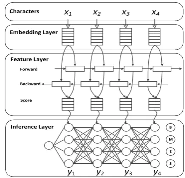
The general architecture of neural CWS could be characterized by three components: (1) a cha-racter embedding layer; (2) feature layers consis-ting of several classical neural networks and (3) a tag inference layer. The role of feature layers is to extract features, which could be either convolution neural network or recurrent neural network. In this

Characters

Embedding Layer

Feature Layer

Inference Layer B

M

E

S

y3

y2

y1 y4

x4

x1 x2 x3

Forward

Backward

Score

Figure 1: General neural architecture for Chinese word segmentation.

paper, we adopt the bi-directional long short-term memory neural networks followed by CRF as the tag inference layer. Figure1illustrates the general architecture of CWS.

2.1 Embedding layer

In neural models, the first step usually is to map discrete language symbols to distributed embed-ding vectors. Formally, we lookup embedding vector from embedding matrix for each character

xi as exi ∈ R

de_{, where d}

e is a hyper-parameter indicating the size of character embedding.

2.2 Feature layers

We adopt bi-directional long short-term memory (Bi-LSTM) as feature layers. While there are nu-merous LSTM variants, here we use the LSTM ar-chitecture used by (Jozefowicz et al.,2015), which is similar to the architecture of (Graves,2013) but without peep-hole connections.

LSTM LSTM introduces gate mechanism and memory cell to maintain long dependency infor-mation and avoid gradient vanishing. Formally, LSTM, with input gatei, output gateo, forget gate fand memory cellc, could be expressed as:

   

ii oi fi ˜ ci

   =

   

σ σ σ ϕ

   

(

Wg|

[

ex_i hi−1

]

+bg

)

, (2)

ci =ci₋1⊙fi+ ˜ci⊙ii, (3)

hi =oi⊙ϕ(ci), (4)

in-dicating the hidden state size. Functionσ(_·) and

ϕ(·)are sigmoid and tanh functions respectively.

Bi-LSTM In order to incorporate information from both sides of sequence, we use bi-directional LSTM (Bi-LSTM) with forward and backward di-rections. The update of each Bi-LSTM unit can be written precisely as follows:

hi =−→hi⊕←−hi, (5)

=Bi-LSTM(exi,

− →

hi−1,←−hi+1, θ), (6)

where−→hiand←−hiare the hidden states at positioni of the forward and backward LSTMs respectively;

⊕is concatenation operation; θ denotes all para-meters in Bi-LSTM model.

2.3 Inference Layer

After extracting features, we employ conditional random fields (CRF) (Lafferty et al.,2001) layer to inference tags. In CRF layer,p(Y|X)in Eq (1) could be formalized as:

p(Y_|X) = ∑ Ψ(Y|X)

Y′_∈LnΨ(Y′|X)

. (7)

Here, Ψ(Y|X) is the potential function, and we only consider interactions between two successive labels (first order linear chain CRFs):

Ψ(Y_|X) = n

∏

i=2

ψ(X, i, yi−1, yi), (8)

ψ(x, i, y′, y) =exp(s(X, i)y+by′y), (9)

whereby′y ∈Ris trainable parameters respective to label pair(y′, y). Score functions(X, i)∈R|L|

assigns score for each label on tagging thei-th cha-racter:

s(X, i) =W⊤_shi+bs, (10)

wherehi is the hidden state of Bi-LSTM at posi-tioni;Ws ∈Rdh×|L|_{andbs ∈} R|L|_{are trainable}

parameters.

3 Multi-Criteria Learning for Chinese Word Segmentation

Although neural models are widely used on CWS, most of them cannot deal with incompatible crite-ria with heterogonous segmentation critecrite-ria simul-taneously.

Inspired by the success of multi-task learning (Caruana, 1997; Ben-David and Schuller, 2003; Liu et al., 2016a,b), we regard the heterogenous

criteria as multiple “related” tasks, which could improve the performance of each other simultane-ously with shared information.

Formally, assume that there areM corpora with heterogeneous segmentation criteria. We referDm as corpusmwithNmsamples:

Dm ={(X_i(m), Y_i(m))}N_i=1m, (11)

whereX_im andY_im denote thei-th sentence and the corresponding label in corpusm.

To exploit the shared information between these different criteria, we propose three sharing models for CWS task as shown in Figure2. The feature layers of these three models consist of a private specific) layer and a shared (criterion-invariant) layer. The difference between three mo-dels is the information flow between the task layer and the shared layer. Besides, all of these three models also share the embedding layer.

3.1 Model-I: Parallel Shared-Private Model

In the feature layer of Model-I, we regard the pri-vate layer and shared layer as two parallel layers. For corpusm, the hidden states of shared layer and private layer are:

h(s)_i =Bi-LSTM(exi,

− →_h(s)

i−1,←−h (s)

i+1, θs), (12)

h(m)_i =Bi-LSTM(exi,

− →

h(m)_i−1,←h−(m)_i+1, θm), (13)

and the score function in the CRF layer is compu-ted as:

s(m)(X, i) =W(m)_s ⊤

[

h(s)_i h(m)_i

]

+b(m)_s , (14)

where W(m)s ∈ R2dh×|L| and b(m)s ∈ R|L| are criterion-specific parameters for corpusm.

3.2 Model-II: Stacked Shared-Private Model In the feature layer of Model-II, we arrange the shared layer and private layer in stacked manner. The private layer takes output of shared layer as input. For corpusm, the hidden states of shared layer and private layer are:

h(_is)=Bi-LSTM(exi,

− →_h(s)

i−1,←−h (s)

i+1, θs), (15)

h(_im)=Bi-LSTM(

[_e

xi

h(_is)

]

,−→h(_i−m₁),←−h(_i+1m), θm) (16)

and the score function in the CRF layer is compu-ted as:

s(m)(X, i) =W(m)_s ⊤h(m)_i +b(m)_s , (17)

CRF

CRF Task A

Task B

X(A)

X(B)

Y(B) Y(A)

(a) Model-I

CRF

CRF Task A

Task B

X(A)

X(B)

Y(B) Y(A)

(b) Model-II

CRF

CRF Task A

Task B

X(A)

X(B)

Y(B) Y(A)

(c) Model-III

Figure 2: Three shared-private models for multi-criteria learning. The yellow blocks are the shared Bi-LSTM layer, while the gray block are the private Bi-Bi-LSTM layer. The yellow circles denote the shared embedding layer. The red information flow indicates the difference between three models.

3.3 Model-III: Skip-Layer Shared-Private Model

In the feature layer of Model-III, the shared layer and private layer are in stacked manner as Model-II. Additionally, we send the outputs of shared layer to CRF layer directly.

The Model III can be regarded as a combination of Model-I and Model-II. For corpusm, the hidden states of shared layer and private layer are the same with Eq (15) and (16), and the score function in CRF layer is computed as the same as Eq (14).

3.4 Objective function

The parameters of the network are trained to max-imize the log conditional likelihood of true labels on all the corpora. The objective functionJsegcan be computed as:

Jseg(Θm,Θs) = M

∑

m=1

Nm

∑

i=1

logp(Y_i(m)|X_i(m); Θm,Θs), (18) whereΘmandΘsdenote all the parameters in pri-vate and shared layers respectively.

4 Incorporating Adversarial Training for Shared Layer

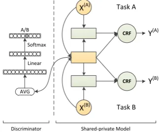
Although the shared-private model separates the feature space into shared and private spaces, there is no guarantee that sharable features do not ex-ist in private feature space, or vice versa. Inspired by the work on domain adaptation (Ajakan et al., 2014;Ganin et al.,2016;Bousmalis et al.,2016), we hope that the features extracted by shared layer is invariant across the heterogonous segmentation criteria. Therefore, we jointly optimize the shared

CRF

CRF Task A

Task B

AVG

Discriminator Shared-private Model

X(A)

X(B)

Y(B) Y(A)

A/B

Softmax

Linear

Figure 3: Architecture of Model-III with adversa-rial training strategy for shared layer. The discri-minator firstly averages the hidden states of shared layer, then derives probability over all possible cri-teria by applying softmax operation after a linear transformation.

layer via adversarial training (Goodfellow et al., 2014).

Therefore, besides the task loss for CWS, we ad-ditionally introduce an adversarial loss to prevent criterion-specific feature from creeping into shared space as shown in Figure3. We use a criterion dis-criminator which aims to recognize which criterion the sentence is annotated by using the shared fea-tures.

Specifically, given a sentenceX with lengthn, we refer to h(s)_X as shared features for X in one of the sharing models. Here, we computeh(s)_X by simply averaging the hidden states of shared layer h(s)_X = _n1 ∑n_i h(s)xi . The criterion discriminator

computes the probability p(_·|X) over all criteria as:

whereΘd_{indicates the parameters of criterion} dis-criminatorWd∈Rdh×M andbd∈RM;Θs deno-tes the parameters of shared layers.

4.1 Adversarial loss function

The criterion discriminator maximizes the cross entropy of predicted criterion distribution p(·|X) and true criterion.

max

Θd J

1

adv(Θd) =

M

∑

m=1

Nm

∑

i=1

logp(m|Xi(m); Θ d

,Θs). (20)

An adversarial loss aims to produce shared fea-tures, such that a criterion discriminator cannot re-liably predict the criterion by using these shared fe-atures. Therefore, we maximize the entropy of pre-dicted criterion distribution when training shared parameters.

max

Θs J

2

adv(Θs) =

M

∑

m=1

Nm

∑

i=1

H(p(m_|X_i(m); Θd,Θs)), (21) where H(p) =₋∑_ipilogpiis an entropy of dis-tributionp.

Unlike (Ganin et al.,2016), we use entropy term instead of negative cross-entropy.

5 Training

Finally, we combine the task and adversarial ob-jective functions.

J(Θ;D) =Jseg(Θm,Θs) +Jadv1 (Θd) +λJadv2 (Θs),

(22) whereλis the weight that controls the interaction of the loss terms and_Dis the training corpora.

The training procedure is to optimize two dis-criminative classifiers alternately as shown in Al-gorithm1. We use Adam (Kingma and Ba,2014) with minibatchs to maximize the objectives.

Notably, when using adversarial strategy, we firstly train 2400 epochs (each epoch only trains on eight batches from different corpora), then we only optimize Jseg(Θm,Θs) with Θs fixed until convergence (early stop strategy).

6 Experiments

6.1 Datasets

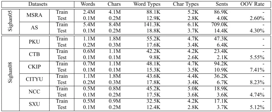
To evaluate our proposed architecture, we experi-ment on eight prevalent CWS datasets from SIG-HAN2005 (Emerson, 2005) and SIGHAN2008 (Jin and Chen,2008). Table2gives the details of the eight datasets. Among these datasets, AS, CI-TYU and CKIP are traditional Chinese, while the

Algorithm 1 Adversarial multi-criteria learning for CWS task.

1: fori= 1;i <=n_epoch;i+ +do

2: # Train tag predictor for CWS

3: form= 1;m <=M;m+ +do

4: # Randomly pick data from corpusm

5: B={X, Y}b₁m ∈ Dm 6: Θs+=α∇ΘsJ(Θ;B)

7: Θm+=α_∇ΘmJ(Θ;B)

8: end for

9: # Train criterion discriminator

10: form= 1;m <=M;m+ +do

11: B={X, Y}bm

1 ∈ Dm 12: Θd+=α∇ΘdJ(Θ;B)

13: end for 14: end for

remains, MSRA, PKU, CTB, NCC and SXU, are simplified Chinese. We use 10% data of shuffled train set as development set for all datasets.

6.2 Experimental Configurations

For hyper-parameter configurations, we set both the character embedding sizedeand the dimensi-onality of LSTM hidden statesdhto 100. The ini-tial learning rateαis set to 0.01. The loss weight coefficientλis set to 0.05. Since the scale of each dataset varies, we use different training batch sizes for datasets. Specifically, we set batch sizes of AS and MSR datasets as 512 and 256 respectively, and 128 for remains. We employ dropout strategy on embedding layer, keeping 80% inputs (20% dro-pout rate).

For initialization, we randomize all parameters following uniform distribution at (₋0.05,0.05). We simply map traditional Chinese characters to simplified Chinese, and optimize on the same cha-racter embedding matrix across datasets, which is pre-trained on Chinese Wikipedia corpus, using word2vec toolkit (Mikolov et al., 2013). Follo-wing previous work (Chen et al.,2015b;Pei et al., 2014), all experiments including baseline results are using pre-trained character embedding with bi-gram feature.

6.3 Overall Results

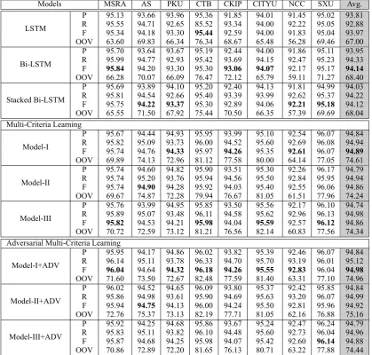
Table 3shows the experiment results of the pro-posed models on test sets of eight CWS datasets, which has three blocks.

Datasets Words Chars Word Types Char Types Sents OOV Rate

Sighan05

MSRA Train 2.4M 4.1M 88.1K 5.2K 86.9K

-Test 0.1M 0.2M 12.9K 2.8K 4.0K 2.60%

AS Train 5.4M 8.4M 141.3K 6.1K 709.0K

-Test 0.1M 0.2M 18.8K 3.7K 14.4K 4.30%

Sighan08

PKU Train 1.1M 1.8M 55.2K 4.7K 47.3K

-Test 0.2M 0.3M 17.6K 3.4K 6.4K

-CTB Train 0.6M 1.1M 42.2K 4.2K 23.4K

-Test 0.1M 0.1M 9.8K 2.6K 2.1K 5.55%

CKIP Train 0.7M 1.1M 48.1K 4.7K 94.2K

-Test 0.1M 0.1M 15.3K 3.5K 10.9K 7.41%

CITYU Train 1.1M 1.8M 43.6K 4.4K 36.2K

-Test 0.2M 0.3M 17.8K 3.4K 6.7K 8.23%

NCC Train 0.5M 0.8M 45.2K 5.0K 18.9K

-Test 0.1M 0.2M 17.5K 3.6K 3.6K 4.74%

SXU Train 0.5M 0.9M 32.5K 4.2K 17.1K

-Test 0.1M 0.2M 12.4K 2.8K 3.7K 5.12%

Table 2: Details of the eight datasets.

performance of Bi-LSTM cannot be improved by merely increasing the depth of networks. In addi-tion, although the F value of LSTM model in (Chen et al.,2015b) is 97.4%, they additionally incorpo-rate an external idiom dictionary.

(2) In the second block, our proposed three mo-dels based on multi-criteria learning boost per-formance. Model-I gains 0.75% improvement on averaging F-measure score compared with Bi-LSTM result (94.14%). Only the performance on MSRA drops slightly. Compared to the baseline results (Bi-LSTM and stacked Bi-LSTM), the pro-posed models boost the performance with the help of exploiting information across these heterogene-ous segmentation criteria. Although variheterogene-ous crite-ria have different segmentation granularities, there are still some underlying information shared. For instance, MSRA and CTB treat family name and last name as one token “宁 泽 涛 (NingZeTao)”, whereas some other datasets, like PKU, regard them as two tokens, “宁 (Ning)” and “泽涛 (Ze-Tao)”. The partial boundaries (before “宁(Ning)” or after “涛(Tao)”) can be shared.

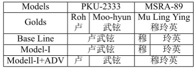
(3) In the third block, we introduce adversarial training. By introducing adversarial training, the performances are further boosted, and Model-I is slightly better than Model-II and Model-III. The adversarial training tries to make shared layer keep criteria-invariant features. For instance, as shown in Table 3, when we use shared information, the performance on MSRA drops (worse than baseline result). The reason may be that the shared parame-ters bias to other segmentation criteria and intro-duce noisy features into shared parameters. When we additionally incorporate the adversarial

stra-tegy, we observe that the performance on MSRA is improved and outperforms the baseline results. We could also observe the improvements on ot-her datasets. However, the boost from the adver-sarial strategy is not significant. The main rea-son might be that the proposed three sharing mo-dels implicitly attempt to keep invariant features by shared parameters and learn discrepancies by the task layer.

6.4 Speed

To further explore the convergence speed, we plot the results on development sets through epochs. Figure4shows the learning curve of Model-I wit-hout incorporating adversarial strategy. As shown in Figure 4, the proposed model makes progress gradually on all datasets. After about 1000 epochs, the performance becomes stable and convergent.

Models MSRA AS PKU CTB CKIP CITYU NCC SXU Avg.

LSTM

P 95.13 93.66 93.96 95.36 91.85 94.01 91.45 95.02 93.81 R 95.55 94.71 92.65 85.52 93.34 94.00 92.22 95.05 92.88 F 95.34 94.18 93.30 95.44 92.59 94.00 91.83 95.04 93.97 OOV 63.60 69.83 66.34 76.34 68.67 65.48 56.28 69.46 67.00

Bi-LSTM

P 95.70 93.64 93.67 95.19 92.44 94.00 91.86 95.11 93.95 R 95.99 94.77 92.93 95.42 93.69 94.15 92.47 95.23 94.33

F 95.84 94.20 93.30 95.30 93.06 94.07 92.17 95.17 94.14

OOV 66.28 70.07 66.09 76.47 72.12 65.79 59.11 71.27 68.40

Stacked Bi-LSTM

P 95.69 93.89 94.10 95.20 92.40 94.13 91.81 94.99 94.03 R 95.81 94.54 92.66 95.40 93.39 93.99 92.62 95.37 94.22 F 95.75 94.22 93.37 95.30 92.89 94.06 92.21 95.18 94.12 OOV 65.55 71.50 67.92 75.44 70.50 66.35 57.39 69.69 68.04 Multi-Criteria Learning

Model-I

P 95.67 94.44 94.93 95.95 93.99 95.10 92.54 96.07 94.84 R 95.82 95.09 93.73 96.00 94.52 95.60 92.69 96.08 94.94 F 95.74 94.76 94.33 95.97 94.26 95.35 92.61 96.07 94.89

OOV 69.89 74.13 72.96 81.12 77.58 80.00 64.14 77.05 74.61

Model-II

P 95.74 94.60 94.82 95.90 93.51 95.30 92.26 96.17 94.79 R 95.74 95.20 93.76 95.94 94.56 95.50 92.84 95.95 94.94 F 95.74 94.90 94.28 95.92 94.03 95.40 92.55 96.06 94.86 OOV 69.67 74.87 72.28 79.94 76.67 81.05 61.51 77.96 74.24

Model-III

P 95.76 93.99 94.95 95.85 93.50 95.56 92.17 96.10 94.74 R 95.89 95.07 93.48 96.11 94.58 95.62 92.96 96.13 94.98

F 95.82 94.53 94.21 95.98 94.04 95.59 92.57 96.12 94.86

OOV 70.72 72.59 73.12 81.21 76.56 82.14 60.83 77.56 74.34 Adversarial Multi-Criteria Learning

Model-I+ADV

P 95.95 94.17 94.86 96.02 93.82 95.39 92.46 96.07 94.84 R 96.14 95.11 93.78 96.33 94.70 95.70 93.19 96.01 95.12

F 96.04 94.64 94.32 96.18 94.26 95.55 92.83 96.04 94.98

OOV 71.60 73.50 72.67 82.48 77.59 81.40 63.31 77.10 74.96

Model-II+ADV

P 96.02 94.52 94.65 96.09 93.80 95.37 92.42 95.85 94.84 R 95.86 94.98 93.61 95.90 94.69 95.63 93.20 96.07 94.99 F 95.94 94.75 94.13 96.00 94.24 95.50 92.81 95.96 94.92 OOV 72.76 75.37 73.13 82.19 77.71 81.05 62.16 76.88 75.16

Model-III+ADV

P 95.92 94.25 94.68 95.86 93.67 95.24 92.47 96.24 94.79 R 95.83 95.11 93.82 96.10 94.48 95.60 92.73 96.04 94.96 F 95.87 94.68 94.25 95.98 94.07 95.42 92.60 96.14 94.88 OOV 70.86 72.89 72.20 81.65 76.13 80.71 63.22 77.88 74.44

Table 3: Results of proposed models on test sets of eight CWS datasets. There are three blocks. The first block consists of two baseline models: Bi-LSTM and stacked Bi-LSTM. The second block consists of our proposed three models without adversarial training. The third block consists of our proposed three models with adversarial training. Here, P, R, F, OOV indicate the precision, recall, F value and OOV recall rate respectively. The maximum F values in each block are highlighted for each dataset.

6.5 Error Analysis

We further investigate the benefits of the propo-sed models by comparing the error distributions between the single-criterion learning (baseline mo-del Bi-LSTM) and multi-criteria learning (Momo-del-I and Model-I with adversarial training) as shown in Figure5. According to the results, we could ob-serve that a large proportion of points lie above diagonal lines in Figure5aand Figure5b, which implies that performance benefit from integrating knowledge and complementary information from other corpora. As shown in Table 3, on the test set of CITYU, the performance of Model-I and its adversarial version (Model-I+ADV) boost from

92.17% to 95.59% and 95.42% respectively.

0 500 1,000 1,500 2,000 2,500 90

92 94 96

epoches

F-value(%) MSRA AS

PKU CTB

CKIP CITYU

NCC SXU

Figure 4: Convergence speed of Model-I without adversarial training on development sets of eight datasets.

40 50 60 70 80 90 100

40 50 60 70 80 90 100

M

u

lt

i-C

ri

te

ri

a

Le

ar

n

in

g

Base Line

(a)

40 50 60 70 80 90 100

40 50 60 70 80 90 100

M

u

lt

i-C

ri

te

ri

a

Le

ar

n

in

g

+

A

d

ve

rs

ar

y

Base Line

(b)

Figure 5: F-measure scores on test set of CITYU dataset. Each point denotes a sentence, with the (x, y) values of each point denoting the F-measure scores of the two models, respectively. (a) is comparison between Bi-LSTM and Model-I. (b) is comparison between Bi-LSTM and Model-I with adversarial training.

7 Knowledge Transfer

We also conduct experiments of whether the shared layers can be transferred to the other related tasks or domains. In this section, we investigate the ability of knowledge transfer on two experi-ments: (1) simplified Chinese to traditional Chi-nese and (2) formal texts to informal texts.

7.1 Simplified Chinese to Traditional Chinese

Traditional Chinese and simplified Chinese are two similar languages with slightly difference on character forms (e.g. multiple traditional charac-ters might map to one simplified character). We investigate that if datasets in traditional Chinese and simplified Chinese could help each other. Ta-ble 5 gives the results of Model-I on 3

traditio-Models PKU-2333 MSRA-89

Golds Roh Moo-hyun Mu Ling Ying_{卢 武铉 穆玲英}

Base Line 卢武铉 穆 玲英

Model-I 卢武铉 穆 玲英

Modell-I+ADV 卢 武铉 穆玲英

Table 4: Segmentation cases of personal names.

Models AS CKIP CITYU Avg.

Baseline(Bi-LSTM) 94.20 93.06 94.07 93.78 Model-I∗ 94.12 93.24 95.20 94.19

Table 5: Performance on 3 traditional Chinese da-tasets. Model-I∗ means that the shared parameters are trained on 5 simplified Chinese datasets and are fixed for traditional Chinese datasets. Here, we conduct Model-I without incorporating adversarial training strategy.

nal Chinese datasets under the help of 5 simpli-fied Chinese datasets. Specifically, we firstly train the model on simplified Chinese datasets, then we train traditional Chinese datasets independently with shared parameters fixed.

As we can see, the average performance is boos-ted by 0.41% on F-measure score (from 93.78% to 94.19%), which indicates that shared features le-arned from simplified Chinese segmentation crite-ria can help to improve performance on traditio-nal Chinese. Like MSRA, as AS dataset is relati-vely large (train set of 5.4M tokens), the features learned by shared parameters might bias to other datasets and thus hurt performance on such large dataset AS.

7.2 Formal Texts to Informal Texts

7.2.1 Dataset

We use the NLPCC 2016 dataset2(Qiu et al.,2016) to evaluate our model on micro-blog texts. The NLPCC 2016 data are provided by the shared task in the 5th CCF Conference on Natural Language Processing & Chinese Computing (NLPCC 2016): Chinese Word Segmentation and POS Tagging for micro-blog Text. Unlike the popular used news-wire dataset, the NLPCC 2016 dataset is collected from Sina Weibo3, which consists of the informal texts from micro-blog with the various topics, such as finance, sports, entertainment, and so on. The information of the dataset is shown in Table6.

2_{https://github.com/FudanNLP/} NLPCC-WordSeg-Weibo

Dataset Words Chars Word Types Char Types Sents OOV Rate Train 421,166 688,743 43,331 4,502 20,135

-Dev 43,697 73,246 11,187 2,879 2,052 6.82%

Test 187,877 315,865 27,804 3,911 8,592 6.98%

Table 6: Statistical information of NLPCC 2016 dataset.

Models P R F OOV

Baseline(Bi-LSTM) 93.56 94.33 93.94 70.75 Model-I∗ 93.65 94.83 94.24 74.72

Table 7: Performances on the test set of NLPCC 2016 dataset. Model-I∗ means that the shared pa-rameters are trained on 8 Chinese datasets (Table 2) and are fixed for NLPCC dataset. Here, we conduct Model-I without incorporating adversarial training strategy.

7.2.2 Results

Formal documents (like the eight datasets in Table 2) and micro-blog texts are dissimilar in many as-pects. Thus, we further investigate that if the for-mal texts could help to improve the performance of micro-blog texts. Table7 gives the results of Model-I on the NLPCC 2016 dataset under the help of the eight datasets in Table2. Specifically, we firstly train the model on the eight datasets, then we train on the NLPCC 2016 dataset alone with shared parameters fixed. The baseline model is Bi-LSTM which is trained on the NLPCC 2016 data-set alone.

As we can see, the performance is boosted by 0.30% on F-measure score (from 93.94% to 94.24%), and we could also observe that the OOV recall rate is boosted by 3.97%. It shows that the shared features learned from formal texts can help to improve the performance on of micro-blog texts.

8 Related Works

There are many works on exploiting heterogene-ous annotation data to improve variheterogene-ous NLP tasks. Jiang et al.(2009) proposed a stacking-based mo-del which could train a momo-del for one specific de-sired annotation criterion by utilizing knowledge from corpora with other heterogeneous annotati-ons. Sun and Wan (2012) proposed a structure-based stacking model to reduce the approximation error, which makes use of structured features such as sub-words. These models are unidirectional aid and also suffer from error propagation problem.

Qiu et al. (2013) used multi-tasks learning fra-mework to improve the performance of POS

tag-ging on two heterogeneous datasets. Li et al. (2015) proposed a coupled sequence labeling mo-del which could directly learn and infer two he-terogeneous annotations. Chao et al. (2015) also utilize multiple corpora using coupled sequence la-beling model. These methods adopt the shallow classifiers, therefore suffering from the problem of defining shared features.

Our proposed models use deep neural networks, which can easily share information with hidden shared layers. Chen et al. (2016) also adopted neural network models for exploiting heterogene-ous annotations based on neural multi-view model, which can be regarded as a simplified version of our proposed models by removing private hidden layers.

Unlike the above models, we design three sharing-private architectures and keep shared layer to extract criterion-invariance features by introdu-cing adversarial training. Moreover, we fully ex-ploit eight corpora with heterogeneous segmenta-tion criteria to model the underlying shared infor-mation.

9 Conclusions & Future Works

In this paper, we propose adversarial multi-criteria learning for CWS by fully exploiting the under-lying shared knowledge across multiple heteroge-neous criteria. Experiments show that our propo-sed three shared-private models are effective to ex-tract the shared information, and achieve signifi-cant improvements over the single-criterion met-hods.

Acknowledgments

References

Hana Ajakan, Pascal Germain, Hugo Larochelle, François Laviolette, and Mario Marchand. 2014. Domain-adversarial neural networks. arXiv preprint arXiv:1412.4446.

S. Ben-David and R. Schuller. 2003. Exploiting task relatedness for multiple task learning. Learning The-ory and Kernel Machinespages 567–580.

Konstantinos Bousmalis, George Trigeorgis, Nathan Silberman, Dilip Krishnan, and Dumitru Erhan. 2016. Domain separation networks. InAdvances in Neural Information Processing Systems. pages 343– 351.

Rich Caruana. 1997. Multitask learning. Machine le-arning28(1):41–75.

Jiayuan Chao, Zhenghua Li, Wenliang Chen, and Min Zhang. 2015. Exploiting heterogeneous annotati-ons for weibo word segmentation and pos tagging. InNational CCF Conference on Natural Language Processing and Chinese Computing. Springer, pages 495–506.

Hongshen Chen, Yue Zhang, and Qun Liu. 2016. Neu-ral network for heterogeneous annotations. Procee-dings of the 2016 Conference on Empirical Methods in Natural Language Processing.

Xinchi Chen, Xipeng Qiu, Chenxi Zhu, and Xuanjing Huang. 2015a. Gated recursive neural network for chinese word segmentation. InProceedings of An-nual Meeting of the Association for Computational Linguistics..

Xinchi Chen, Xipeng Qiu, Chenxi Zhu, Pengfei Liu, and Xuanjing Huang. 2015b. Long short-term me-mory neural networks for chinese word segmenta-tion. InEMNLP. pages 1197–1206.

Ronan Collobert and Jason Weston. 2008. A unified architecture for natural language processing: Deep neural networks with multitask learning. In Procee-dings of ICML.

Thomas Emerson. 2005. The second international chi-nese word segmentation bakeoff. InProceedings of the fourth SIGHAN workshop on Chinese language Processing. volume 133.

XIA Fei. 2000. The part-of-speech tagging guide-lines for the penn chinese treebank (3.0). URL: http://www. cis. upenn. edu/˜ chinese/segguide. 3rd. ch. pdf .

Yaroslav Ganin, Evgeniya Ustinova, Hana Ajakan, Pascal Germain, Hugo Larochelle, François La-violette, Mario Marchand, and Victor Lempitsky. 2016. Domain-adversarial training of neural net-works. Journal of Machine Learning Research 17(59):1–35.

Ian Goodfellow, Jean Pouget-Abadie, Mehdi Mirza, Bing Xu, David Warde-Farley, Sherjil Ozair, Aaron Courville, and Yoshua Bengio. 2014. Generative ad-versarial nets. In Advances in Neural Information Processing Systems. pages 2672–2680.

Alex Graves. 2013. Generating sequences with recurrent neural networks. arXiv preprint arXiv:1308.0850.

W. Jiang, L. Huang, and Q. Liu. 2009. Automatic adap-tation of annoadap-tation standards: Chinese word seg-mentation and POS tagging: a case study. In Pro-ceedings of the Joint Conference of the 47th Annual Meeting of the ACL and the 4th International Joint Conference on Natural Language Processing. pages 522–530.

G. Jin and X. Chen. 2008. The fourth international chinese language processing bakeoff: Chinese word segmentation, named entity recognition and chinese pos tagging. InSixth SIGHAN Workshop on Chinese Language Processing. page 69.

Rafal Jozefowicz, Wojciech Zaremba, and Ilya Sutske-ver. 2015. An empirical exploration of recurrent net-work architectures. InProceedings of The 32nd In-ternational Conference on Machine Learning.

Diederik Kingma and Jimmy Ba. 2014. Adam: A method for stochastic optimization. arXiv preprint arXiv:1412.6980.

John D. Lafferty, Andrew McCallum, and Fernando C. N. Pereira. 2001. Conditional random fields: Probabilistic models for segmenting and labeling se-quence data. InProceedings of the Eighteenth Inter-national Conference on Machine Learning.

Zhenghua Li, Jiayuan Chao, Min Zhang, and Wenliang Chen. 2015. Coupled sequence labeling on hetero-geneous annotations: Pos tagging as a case study. In Proceedings of the 53rd Annual Meeting of the As-sociation for Computational Linguistics and the 7th International Joint Conference on Natural Language Processing.

Zhenghua Li, Jiayuan Chao, Min Zhang, and Jiwen Yang. 2016. Fast coupled sequence labeling on he-terogeneous annotations via context-aware pruning. InProceedings of EMNLP.

Pengfei Liu, Xipeng Qiu, and Xuanjing Huang. 2016a. Deep multi-task learning with shared memory. In Proceedings of the 2016 Conference on Empirical Methods in Natural Language Processing.

Pengfei Liu, Xipeng Qiu, and Xuanjing Huang. 2016b. Recurrent neural network for text classification with multi-task learning. InProceedings of International Joint Conference on Artificial Intelligence.

Tomas Mikolov, Kai Chen, Greg Corrado, and Jef-frey Dean. 2013. Efficient estimation of word representations in vector space. arXiv preprint arXiv:1301.3781.

Wenzhe Pei, Tao Ge, and Chang Baobao. 2014. Max-margin tensor neural network for chinese word seg-mentation. InProceedings of ACL.

Xipeng Qiu, Peng Qian, and Zhan Shi. 2016. Overview of the NLPCC-ICCPOL 2016 shared task: Chinese word segmentation for micro-blog texts. In Interna-tional Conference on Computer Processing of Orien-tal Languages. Springer, pages 901–906.

Xipeng Qiu, Jiayi Zhao, and Xuanjing Huang. 2013. Joint chinese word segmentation and pos tagging on heterogeneous annotated corpora with multiple task learning. InEMNLP. pages 658–668.

Weiwei Sun and Xiaojun Wan. 2012. Reducing ap-proximation and estimation errors for chinese lexical processing with heterogeneous annotations. In Pro-ceedings of the 50th Annual Meeting of the Associ-ation for ComputAssoci-ational Linguistics: Long Papers-Volume 1. pages 232–241.

S. Yu, J. Lu, X. Zhu, H. Duan, S. Kang, H. Sun, H. Wang, Q. Zhao, and W. Zhan. 2001. Processing norms of modern Chinese corpus. Technical report, Technical report.