Functionals of order statistics and their multivariate concomitants with application to semiparametric estimation by nearest neighbours

Munich Personal RePEc Archive

Functionals of order statistics and their

multivariate concomitants with

application to semiparametric estimation

by nearest neighbours

Chu, Ba and Huynh, Kim and Jacho-Chavez, David

Carleton University, Bank of Canada, Emory University

2013

Online at

https://mpra.ub.uni-muenchen.de/79670/

Functionals of Order Statistics and their Multivariate Concomitants

with Application to Semiparametric Estimation by Nearest Neighbors

Ba M. Chu∗ Carleton University

Kim P. Huynh† Bank of Canada

David T. Jacho-Ch´avez‡ Emory University

Abstract

This paper studies the limiting behavior of general functionals of order statistics and their mul-tivariate concomitants for weakly dependent data. The asymptotic analysis is performed under a conditional moment-based notion of dependence for vector-valued time series. It is argued, through analysis of various examples, that the dependence conditions of this type can be effectively implied by other dependence formations recently proposed in time-series analysis, thus it may cover many existing linear and nonlinear processes. The utility of this result is then illustrated in deriving the asymptotic properties of a semiparametric estimator that uses thek-Nearest Neighbor estimator of the inverse of a multivariate unknown density. This estimator is then used to calculate consumer surpluses for electricity demand in Ontario for the period 1971 to 1994. A Monte Carlo experiment also assesses the efficacy of the derived limiting behavior in finite samples for both these general functionals and the proposed estimator.

Keywords: Order statistics; multivariate concomitant;k-nearest neighbor; semiparametric estima-tion; consumer surplus calculation.

AMS 2000 subject classification: 62G30; 62H12; 62G05; 62G07; 62E20

∗_{Department of Economics, Carleton University, B-857 Loeb Building, 1125 Colonel By Drive, Ottawa, ON K1S 5B6,}

Canada. E-mail: ba [email protected]. Web Page: http://http-server.carleton.ca/˜bchu/

†_{Bank of Canada, 234 Wellington Street, Ottawa, Ontario K1A 0G9, Canada. E-mail: [email protected]. Web Page:}

http://www.huynh.tv/

‡_{Corresponding Author: Department of Economics, Emory University, Rich Building 306, 1602 Fishburne Dr., Atlanta,}

1

Introduction

Let (X_t⊤, Yt)⊤ be a RN+1-valued time series process on the probability space (Ω,A,P). Let Y(1) < · · ·< Y_(t)<_{· · ·}< Y_(T) be the order statistics; andX_[t] paired withY_(t)is called the concomitant of the

t-th order statistics in the sample {X_t⊤, Yt}Tt=1.

The use of order statistics and their multivariate concomitants often arises in various statistical problems. For example, selection procedures dictates that s-observations (< T) are chosen on the basis of their Y-values. Then the corresponding X-values represent their associated characteristics. Alternatively Y might represent the score on a screening test andX can represent the score of a later test. Concomitants have also proven useful in the estimation of parameters using doubly censored samples, i.e. Watterson (1958) in estimating means, Barnett et al. (1976) in estimating correlations, andStokes(1977) in ranked set. The properties of concomitants have been studied extensively by many authors, and important contributions include but are not limited toDavid and Galambos(1974), Yang (1977), Nagaraja and David (1994), Khaledi and Kochar (2000) and Arnold et al. (2009), inter alios. The study of concomitants as an important class of statistics has been more recently reviewed byDavid and Nagaraja (1998).

A significant line of work has focused on the asymptotic distribution of general functions of concomi-tants. For example,Yang(1981a,b) proved the asymptotic normality, under mild regularity conditions, of functionals of the form

1

n

n

X

i=1

J

i n+ 1

W[i]

and

1

n

n

X

i=1

J

i n+ 1

h(Z(i), W[i]),

where J(_·) is a bounded, smooth score function which may depend on n, and h(z, w) is a known

R_{−valued function. Stute (1993) established a functional central limit theorem for U-functions of}

concomitants defined as

1

n(n₋1) X

1≤i6=j≤[nt]

K(W_[i], W_[j]),

where K(_·,_·) is any symmetric second-order U-kernel. Previous research have used the independent and identically distributed (i.i.d.) assumption in their execution. The notable exceptions are Puri and Tran (1980), Wu (1988), and Tran and Wu (1993). Specifically, Wu (1988) and Tran and Wu (1993) established the asymptotic theory for linear combinations of functions of order statistics (or

L-estimates, as termed by Serfling, 1980, Chapter 8) for nonstationary time series. This assumption is often too strong in applications where data is collected sequentially over time.

Therefore, this paper studies the limiting behavior of general functionals of ordered statistics and their multivariate concomitants with dependent data. In particular, we prove the √T-asymptotic normality, under fairly mild regularity conditions, of functionals such as

T_{T =} 1

T

T

X

t=1

where J(_·) is a bounded smooth score function and h(x, y) is some R_{-valued known function of}

(x⊤, y)⊤∈RN+1_.

Studying the limiting properties of statistics such as (1.1) is important, because its usage in semi-parametric estimation can avoid the presence of random denominators and the usage of trimming functions altogether. For example, consider the Single Index model which is widely studied in the Statistics literature, see, e.g., Ichimura (1993), H¨ardle et al. (1993), Carroll et al. (1997), inter alia. Let _{(Y_t∗,Z_t∗⊤,X_t∗⊤)_}T

t=1 denote a vector-valued time series with the contemporaneous dependence

generated by the partially linear single-index model

Y_t∗ =g(Z_t∗⊤α) +X_t∗⊤β+ǫt, (1.2)

whereZ_t∗andX_t∗are random covariate vectors;g(·) represents an unknown, possibly non-differentiable, function; ǫdenote i.i.d. mean-zero random errors, which are independent of (Z_t∗⊤,X_t∗⊤)⊤; and α and

β are the unknown finite-dimensional parameters to be estimated. The Semiparametric Least Squares (SLS) estimator minimizesQT(α⊤,β⊤)=. PTt=1{Yt∗−bg(Zt∗⊤α;β)−Xt∗⊤β}2,wherebg(Zt∗⊤α;β)

repre-sents the Nearest Neighbor (NN) regression function estimator ofg(Z_t∗⊤α), which can then be written in a form congruent with Eq. (1.1) as follows: Let Yt(α)=. Zt∗⊤α and Wt(β)=. Xt∗⊤β,

b

g(Yt(α);β)=.

1 (T₋1)hT

T_X−1

s=1

[Y_[∗_s]−W[s](β)]K

FT(Yt(α))−s/(T−1)

hT

,

where FT(·) is the empirical distribution function; K(·) is a kernel (weight) function; and X[s](β) =.

(Y_[∗_s], W[s](β)) denotes a vector of the concomitants of the order statistics Y(s)(α) in the sample {(Y₁∗, W1(β), Y1(α)), . . . ,(Yt∗−1, Wt−1(β), Yt−1(α)),(Yt∗+1, Wt+1(β), Yt+1(α)), . . . ,(YT∗, WT(β), YT(α))}.

Stute (1984) shows that in the i.i.d. case, the asymptotic behavior ofg_b(y;β) is the same as that of

b

g∗(y;β) = 1

T−1

T_X−1

s=1

JT(s/(T −1)){Y_[s∗_]−W[s](β)},

where JT (s/(T −1)) =. h−T1K((F(y)−s/(T −1))/hT). Therefore the statistics gb∗(y;β) becomes a

special case of (1.1) with a sample size-varying score function, JT(·). Unlike Ichimura’s (1993) SLS

estimator, the NN regression function estimator contains no random denominator, and no trimming function is needed. However, the non-differentiability of the objective functionQT(α⊤,β⊤) poses many

technical challenges to the derivation of the asymptotic properties of the implied SLS estimator of (1.2) which are beyond the scope of this paper.

Instead, the results of this paper are applied here to study the asymptotic properties of a semipara-metric k-Nearest Neighbor (k-NN) based estimators of objects such as:

θ0 =

Z

x_∈X

E[Y_|X =x]dx=E

Y f(X)

, (1.3)

whereX is some subset in the support of the multivariate densityf(X). Note that, without any loss of generality, assume that X equals the whole support of f(X). Let Supp(f) = _{x _∈ RN _{: f(x) ≥}

In Economics, the object E[Y_|X =x] could represent nonparametric demand or supply functions for a product. In which case quantities such as θ0 can be used to calculate consumer or producer

surplus. The latter are paramount in Microeconomic theory. Recently, the asymptotic properties of various estimators of (1.3) whenN _≥1 has been studied by Lewbel and Schennach (2007), Jacho-Ch´avez(2008),Chu and Jacho-Ch´avez(2012), andLu et al.(2012) under a variety of sampling schemes. A semiparametric estimator that utilizes the k-NN multivariate density estimator of f(_·) is discussed in this paper. This density estimator was first proposed by Loftsgaarden and Quesenberry (1965). Pointwise consistency and asymptotic normality of the k-NN density estimator have been established under various data generating processes: see Moore and Yackel (1977a,b) for i.i.d. samples, Boente and Fraiman(1988,1990) for mixing processes and Tran and Yakowitz (1993) and Li and Tran(2009) for mixing random fields.

The object of interest is thek-NN density in the aforementioned papers, but in the proposed semi-parametric estimator the inverse of thek-NN multivariate density estimator is used instead. The proof of asymptotic normality for this semiparametric estimator, therefore, requires strong consistency of the inverse k-NN multivariate density estimator, which is established here under a fairly mild regularity condition involving a random dependence coefficient. Other estimators using the nearest-neighbors technique in semiparametric problems includeRobinson(1987,1995) and references therein.

Our method of proof can be viewed as a combination of the Gˆateaux differential (see, e.g., Koroljuk and Borovskich,1994, p. 48) and the martingale approximation approach developed inGordin(1969), Philipp and Stout (1975) and Wu and Woodroofe (2004). These are commonly used methods to establish central limit theorems involving stationary data. Theoretically, another contribution is the introduction of a new method of quantifying the notion of contemporaneous dependence for RN+1

-valued processes. In particular, it can be shown that the proposed dependence conditions are related to conditional mixing concepts, as introduced byRao (2009), and random dependence coefficients, as independently proposed byBickel and B¨uhlmann(1999) and Dedecker and Prieur(2005).

2

Basic Notations, Definitions, and Examples

2.1 Basic Notations and Definitions

Let (Ω,_A,P_{) be a probability space, which is sufficiently rich to accommodate (X}⊤_{, Y) and T be a}

measure-preserving, bijective and bimeasurable mapping from Ω onto itself. Let I denote the Borel algebra of invariant sets A _{∈ A} such that _T−1_{A = A. If all the elements of I are of measure 0 or}

1, then a sequence of random variables, (X⊤, Y), defined on (Ω,A,P_{) is said to be ergodic. Define}

a strictly stationary vector-valued sequence of random variables, (X_t⊤, Yt), which can be represented

as Xt =K◦ Tt = K(Ttω) and Yt =H◦ Tt = H(Ttω) for all ω ∈ Ω, where K is a N-dimensional

vector of Borel functions and H is a scalar Borel function. This formulation allows stationary causal processes. Let ǫt = (ǫ1,t, ǫ2,t, . . . , ǫN,t, ǫN+1,t) denote a [N+1]-dimensional vector of i.i.d. random

noises, Xit =Ki(. . . , ǫi,t−1, ǫi,t) for i = 1, . . . , N, and Yt =H(. . . , ǫN+1,t−1, ǫN+1,t). Then (Xt⊤, Yt) is

a causal process, thus naturally falls into the framework; and indeed Yt depends on the filtration of

(X0, . . . ,XT) via the filtration of Xt. We emphasize that the class of causal processes is rather vast

because all time series models used in practice (scalar, vector, or functional) have this representation (cf. Tong, 1990).

For every i _∈ 1, . . . , N, let _Ft,Xi = σ(Xi,s, s ≤ t) = T−tF0,Xi and FXti = σ(Xi,s, s ≥ t) =

Tt_F0

,Xi be Borel algebras generated by (Xi,0, . . . , Xi,t) and (Xi,t, . . . , Xi,T) respectively. Let Ft =

σ (Xs, Ys), s ≤ t = T−tF0 be he smallest σ-algebra in the product Borel algebra, Ft,X1 ⊗ Ft,X2 ⊗

· · · ⊗ Ft,XN ⊗ Ft,Y, generated by {(X0⊤, Y0)⊤, , . . . ,(Xt⊤, Yt)⊤}; F

t _{= σ (X}

s, Ys), s ≥ t = TtF0

represents the smallestσ-algebra in the product Borel algebra,_FXt_{1⊗ FX}t_{2⊗ · · · ⊗ FX}t_{N⊗ FY}t, generated by _{(X_t⊤, Yt)⊤, . . . ,(X_T⊤, YT)⊤}; Ft,X = σ(X_s, s ≤ t) = T−tF0_,X is the smallest σ-algebra in the

product Borel algebra, Ft,X1 ⊗ Ft,X2 ⊗ · · · ⊗ Ft,XN, generated by (X0, . . . ,Xt); F

t

X = σ(Xs, s ≥

t) =_Tt_F0

,X represent the smallest σ-algebra in the product Borel algebra, F_Xt

1 ⊗ F

t

X2 ⊗ · · · ⊗ F

t XN, generated by (Xt, . . . ,XT);Ft,Y =σ(Ys, s≤t) =T−tF0,Y is a Borel algebra generated by (Y0, . . . , Yt);

FYt = σ(Ys, s ≥ t) = TtF0,Y is a Borel algebra generated by (Yt, . . . , YT); FX_t = σ(X_t) represents

the smallest σ-algebra in the product Borel algebra, _FX1,t ⊗ FX2,t ⊗ · · · ⊗ FXN,t, generated by Xt;

FYt = σ(Yt) is a Borel algebra generated by Yt, while F(y|I) is the invariant distribution of Yt, limτ−→∞P(Yτ ≤ y|Y0 ∈ I), where I represents the invariant sets with Borel algebra consisting of

probability measures 0 or 1. The continuity of the following probability distribution functions: F(x),

F(y), and F(x, y) will be assumed throughout this paper – so that ties among the X and Y-variates can be neglected in probability. Finally the quantity _kA_kp is the Lp-norm of A, i.e. {E[|A|p]}1/p;

kAkp,I is the Lp-norm of A conditional on I, i.e. {E[|A|p|I]}1/p. Note that it is possible to simplify

the reading by assuming that _I=_{Ω,_∅}; in this case, any_I-measurable random variable will become a constant, i.e. E[A_|I] =E[A] and E[A_|Y =y,_I] =E[A_|Y =y].

2.2 Examples

For simplicity, we set N = 1 and let ξt denote an i.i.d. mean-zero random variable in the following

• Moving Average (MA) model,Xt=P∞i=0θiξt−i, whereθi are MA coefficients.

• Bilinear (BILINEAR) model, Xt =aXt−1+ξt+bXt−1ξt, where aand b take their values on R,

see, e.g.,Tong (1990).

• Generalized Autoregressive Conditional Heteroskedasticity (1,1) (GARCH) model, Xt = σtξt

withσ2

t =ω+αXt2−1+βσt2−1, whereω,αand β take their values on R.

We now introduce three examples that will serve as illustrations on how a wide range of popular d.g.p.’s satisfy the main assumptions stated below in Section 3.

Example 1: Yt=Xtǫt, whereǫtare i.i.d. mean-zero random variables independent ofXt, andXt can

admit one of the d.g.p.’s above.

Example 2: Yt = XtZt, where Zt is a mean-zero stochastic process that can also follow one of the

above d.g.p.’s, where Zt is independent ofXt.

Example 3: Yt=Xt+Zt, where Zt is as in the Example 2 above.

It will be shown in the next section that the required conditions in the paper are satisfied in these 3 examples. Example 1 is the base of our numerical experimentation in Section 4.1.

3

Assumptions and Main Results

Expressing (1.1) as a functional of empirical distribution functionsFT, yields

T_{(FT) =} 1

T

T

X

t=1

J(t/T)h(X_[t], Y(t))

=

T

X

t=1

J(FT(Y(t)))h(X[t], Y(t))FT(X[t+1], Y(t+1))−FT(X[t], Y(t))

= Z

RN+1

J(FT(y))h(x, y)dFT(x, y),

where FT(y) is the empirical distribution of y and FT(x, y) is the joint empirical distribution of

(X⊤, Y)⊤. Similarly, letmh(y;I)=. E[h(X, Y)|Y =y,I] and mh(y)=. E[h(X, Y)|Y =y].

The following regularity conditions are introduced to facilitate our theoretical development:

A1 Moment Bounds:

For a given integer,p >1, max_{kh(X0, Y0)kp,I,kh(X0, Y0)k2p/(p−1),I}<∞.

A2 Conditional Moments:

(a) m′_h(Y0;I)

_p∗_,I <∞, where m ′

h(·;I) is the first derivative ofmh(·;I).

(b) limτ−→∞supy|P(Yτ ≤y|FY0)−F(y|I)|

q∗_,I = 0, where p∗ and q∗ are such integers that 1/p∗+ 1/q∗ = 1 + (p₋1)/p.

(a) P∞_τ=1kmh(Yτ;F0)−mh(Yτ;I)k_2,F0

p/(p−1),I <∞.

(b) P∞_τ=1kE[h(Xτ, Yτ)h(X0, Y0)|Fτ,Y,I]−mh(Yτ;I)mh(Y0;I)k_p/(p−1),I <∞.

It is helpful to note at this point that, for a scalar-valued Xt, the statistics defined by Eq. (1.1) can

also be represented asT_{(FT) =} 1

T

PT

t=1J(t/T)h(X(t), Y[t]). Accordingly, we shall replacemh(Y;I) and

mh(Y;F0) in AssumptionsA1,A2 and A3 withmh(X;I) and mh(X;F0) respectively.

Remark 3.1. AssumptionA1 entails that moments of the functionh(·,·) are bounded up to a certain order, e.g. any p > 1 can be used depending on what is needed. This mild moment-type condition is often employed to obtain many central limit theorems and invariance principles, i.e. Lyapunov’s central limit theorem. As for AssumptionA2, conditionA2ais automatically fulfilled by any Lipschitz continuous function,mh(·), though this condition does not imply Lipschitz continuity. ConditionA2b

entails asymptotic weak independence (in the ergodic sense) of the random processYt. This condition

is quite close in spirit to the mixing characteristic introduced byRinott and Rotar(1999, p. 613); rather than conditioning the sum of random elements belonging to a ‘past’ Borel algebra on a ‘future’ Borel algebra, we condition a ‘future’ random element on a ‘past’ Borel algebra. ConditionA2bmay be weaker than the usual mixing conditions (see, e.g., Bradley, 1986 for definition of various mixing concepts). For example, by virtue of the covariance inequality for strong mixing random variables (Ibragimov, 1962), one can verify that, for stationary ergodic processes,sup_y|P(Yτ ≤y|F0)−F(y)|

q∗≤2(21/q ∗

+

1)α1τ/q∗−1/r∗ for somer∗ ≥q∗ ≥1, whereατ representsRosenblatt’s (1956a) strong mixing coefficient.

Hence, strong mixing implies Condition A2b. Indeed, many causal processes used in practice, e.g. stationary and ergodic Markov chains, have been shown to satisfy this condition (see, e.g., Pham and Tran,1985,Pham,1986, among many others).

Over the past decades, many approaches have been proposed to formalize weak dependence. In this context, we now discuss how the notion of weak dependence introduced here compares to other existing ones. Perhaps, the most popular are the strong mixing property and its variants like β, φ, ρ and ψ

mixing coefficients, which were developed in the seminal papers ofRosenblatt (1956a) and Ibragimov (1962). The general idea is to measure the maximal dependence between two events pertaining to the backward σ₋ algebra _Ft and the forward σ− algebra Ft+m, respectively. The memory is fading as

this maximal dependence decays to zero, as m increases to infinity. For example, the strong mixing dependence is formalized by

αm = sup A∈Ft

B∈Ft+m

|P(A_∩B)₋P(A)P(B)_|.

A sequence is α₋mixing if αm tends to zero for a sufficiently large m. Recently, Rao (2009) has

introduced the concept of conditional strong mixing, i.e. let M be a σ−algebra of A, a sequence is said to be conditionally strong mixing if there exists a nonnegative _M− measurable random variable

α∗_m(_M) converging to zero a.s. as m goes to infinity, such that

In Section 3.3 below we shall show that, for stationary and ergodic processes, _{X_t⊤, Yt}, the Ces`aro

summability of theconditional strong mixing coefficientα∗_m(M) effectively implies ConditionA3b, but not vice versa.

Although many results have been established for strongly mixing sequences, see e.g. Bradley(2007) and Rio (2000), many classes of time series have been shown not to satisfy these conditions, i.e. An-drews(1984). Therefore, Bickel and B¨uhlmann (1999) andDedecker and Prieur (2005) independently introduced a new concept of weak dependence. Their notion of weak dependence makes explicitly the asymptotic independence between ‘past’ and ‘future’. Roughly speaking, the covariance between measurable functions of the ‘past’ and ‘future’ becomes small as the distance between the ‘past’ and the ‘future’ is large. The decay rate of this covariance is measured through the Lp-distance between

the conditional expectation of a Lipschitz function,g(_·), of a Lp-integrable random variable, X, given

Mand the expectation of g(X). Thus the_M−measurable randomθ₋coefficient is defined as

θp(M) = sup

n

kE[g(X)_|M]₋E[g(X)]_kp, for some functiong_∈Λ(1)o,

where Λ(1) denotes the class of Lipschitz functions with the Lipschitz coefficient at most equal to one. The regularity conditions A3a and A3b essentially imply that the dependence coefficient of θ -type is Ces`aro summable. Here the σ-algebra _M contains two sub σ-algebras, _FYτ and F0, and an important difference being that the functions mh(·) and h(·) in the above conditions may not need to

be Lipschitzian.

An alternative approach to define weak dependence is based on a martingale projection, _Pt(X) =

E[X|Ft]−E[X|Ft−1]. In the context where sequences,Xt, are stationary and ergodic Markov chains,

Wu (2005, 2007) has employed some regularity conditions regarding the Ces`aro summability of the

Lp−norm of Pt(X) and successfully proved strong invariance principles with nearly optimal bounds.

Wu (2007) also validates that these regularity conditions can be directly inferred from the Ces`aro summability of an input/output dependence measure, which is defined as theLp distance between the

conditional expectation of the Markov chain Xt=g(. . . , ǫt−1, ǫt) for some i.i.d. (ǫt)t∈Z and the condi-tional expectation of a decoupled sequence of Xt. In Section 3.1, we demonstrate that by taking into

account the Ces`aro summability of the Lp−norm of a conditional input/output dependence measure

the asymptotic normality of the statistics (1.1) can be established. As a result, Corollary3.1is a special case of Theorem3.1 because AssumptionB3below explicitly implies Assumption A3.

We shall now demonstrate that the d.g.p.’s provided in Section 2.2can fulfill AssumptionsA1-A3.

Example 1 (continued): For ease of derivation, we take the function h(x, y) = (xy)2. Since _Ft =

Ft,Y =. σ((Xs, ǫs) :s≤t), Assumption A1 then becomes

max_kǫ2_0kpkX04kp,kǫ20k2p/(p−1)kX04k2p/(p−1) <∞. (3.1)

ConditionA2a is equivalent to

ǫ2_0p∗

X₀3_p∗ <∞. (3.2) It is straightforward to check that _kmh(Xτ;F0)−mh(Xτ)k2,F0 = 0 andE[h(X0, Y0)h(Xτ, Yτ)|Fτ,X]−

• MA: The MA coefficients θi must be chosen so as to verify (3.1) and (3.2). In addition, if

limτ→∞P∞t=τ(

P_∞

i=t|θi|) δ/(1+δ)

= 0, whereδ is some positive generic constant, then Xt satisfies

the absolutely-regular mixing condition (Pham and Tran, 1985). The absolute regularity then implies Condition A2b.

• BILINEAR: The stationarity condition is a2 +b2 < 1 (see Tong (1990, p. 159)). Therefore the existence of higher-order moments of ǫ0 will validate (3.1) and (3.2). Pham (1986) shows

that, under some regularity conditions, Xt is geometrically ergodic. This automatically implies

ConditionA2b.

• GARCH: If E[log(αξ2

t +β)] < 0, then this GARCH(1,1) model has a non-anticipative strictly

stationary solution, which also satisfies the geometrically absolutely-regular mixing condition (see Francq and Zako¨ıan,2010, p. 71). Since absolute regularity is stronger than strong mixing, ConditionA2b is validated.

Example 2 (continued): Defineh(x, y) =xy. Assumption A1 then becomes

max_kX₀2Z_0kp,kX02Z0k2p/(p−1) <∞. (3.3)

Meanwhile, Condition A2a is fulfilled because of mh(X0) = 0. Also, in view of Example 1, the

various representations of Xt satisfy Condition A2b. We shall now verify Assumption A3: Since

Fτ = Fτ,Y =. σ((Xs, Zs) :s≤τ), it then follows that mh(Xτ;F0) = Xτ2E[Zτ|Xτ,F0] = Xτ2E[Zτ|Z0]

becauseZ is independent of X. Therefore, an application of H¨older’s inequality yields

kmh(Xτ;F0)−mh(Xτ)k2,F0

p/(p−1) =

X_τ2_2,F

0E[Zτ|Z0]

p/(p−1) ≤ X_τ2_2,

F0

p∗ 1

kE[Zτ|Z0]kq∗ 1

≤ X_τ41_p/∗2 1/2k

E[Zτ|Z0]kq∗ 1, wherep∗₁>2 and q₁∗>1 such that 1/p∗₁+ 1/q∗₁ = (p₋1)/p; and

kE[h(X0, Y0)h(Xτ, Yτ)|Fτ,X −mh(Xτ)mh(X0)k_p/(p−1) ≤ X02Xτ2

_p/(p

−1)E[Z0Zτ]

≤ X₀2_2p/(p−1)X_τ2_2p/(p−1)|E[Z0Zτ]|.

Assuming that the coefficients in the time-series models, defined in Example 1, ofXtensure thatXtis

strictly stationary and maxn_kX₀2_kp,

X₀2_2p/(p

−1),

X_τ4_p∗

1/2 o

<_∞, AssumptionA3is thus essentially weaker than

max (_∞

X

τ=1

kE[Zτ|Z0]k_q∗ 1,

∞

X

τ=1

|E[Z0Zτ]|

)

<∞. (3.4)

An application of covariance inequalities for mixing random variables (see, e.g.,Truong and Stone 1992 and Ibragimov 1962) yields

∞

X

τ=1

kE[Zτ|Z0]k_q∗

1 ≤ 2(2

1/q∗

1 + 1)kZ0k

r∗ 1

∞

X

τ=1

α1/q∗1−1/r1∗

τ , where r1∗≥q∗1 ≥1,

∞

X

τ=1

|E[Zτ|Z0]| ≤ 8kZ0kp∗ 2kZτkq

∗ 2

∞

X

τ=1

α1−1/p∗2−1/q∗2

We shall now establish that Conditions (3.3) and (3.4) indeed holds under the various d.g.p. ofZt.

• MA: Zt is strong mixing with ατ = O P∞t=τ+1Gt(r)1/(1+r), where, for either an even

pos-itive integer, r, or 0 < r _≤ 2, Gt(r) =.

2P∞_i=t|θi|r, r≤2,

2r−1₍P∞

i=tθ 2 i)

r/2

, r≥2. (see Davidson, 1994,

Theo-rem 14.9, for sufficient conditions pertaining to this result). Therefore, the MA coefficients

θi must be chosen so as to warrant the existence of the higher-order moments of Zt such

that maxnP∞_τ=1 P∞_t=τ+1Gt(r)1/(1+r)1/q

∗ 1−1/r1∗

,P∞_τ=1 P∞_t=τ+1Gt(r)1/(1+r)1−1/p

∗ 2−1/q∗2o

<_∞, which then validates Conditions (3.3) and (3.4).

• BILINEAR: Geometric ergodicity implies absolute regularity with a geometric convergence rate, which is in turn stronger than strong mixing. Therefore, in view of Example 1, we obtain

ατ =O(ℓτ) for some 0< ℓ <1. It then follows that, ifq1∗,r∗1,p∗2 andq∗2 are chosen in such a way

that maxℓ1/q1∗−1/r1∗, ℓ1−1/p∗2−1/q2∗ <1 so conditions (3.3) and (3.4) are validated.

• GARCH: The GARCH(1,1) process also satisfies the absolutely-regular mixing condition with a geometric convergence rate. The verification of Conditions (3.3) and (3.4) can be done in exactly the same way as for the bilinear model.

Example 3 (continued): Defineh(x, y) =xy, it is immediate to obtain via H¨older’s inequality that:

kmh(Xτ;F0)−mh(Xτ)k2,F0

p/(p−1) ≤

X_τ21_p/∗2

1/2k

E[Zτ|Z0]kq∗ 1 ,

kE[h(X0, Y0)h(Xτ, Yτ)|Fτ,X −mh(Xτ)mh(X0)k_p/(p−1) ≤ kX0k2p/(p−1)kXτk2p/(p−1)|E[Z0Zτ]|.

Therefore, Assumptions A1,A2, and A3can be easily verified for all d.g.p. as in Example 2.

Prior to stating the first theorem of this paper, it is necessary to define the following martin-gale difference sequence: W_t∗ =. P∞_s=t{E[Ws|Ft]−E[Ws|Ft−1]}, where Wt = J(F(Yt|I)){h(Xt, Yt)−

mh(Yt|I)} −RRJ(F(y|I)){I(Yt ≤y)−F(y|I)}dmh(y|I), and I(·) is the standard indicator function. The following theorem states the main result of the paper.

Theorem 3.1. Suppose that Assumptions A1,A2, and A3hold. Then

√

T(T_(FT)−T_(F))=W_{⇒ N 0, σ}2_{W(I), (3.5)}

where σ2_W(I) =E[W₁∗2|I] =E[W₀2|I] + 2P∞_s=1E[W0Ws|I].

3.1 Stationary Causal Processes

Suppose that (X_t⊤, Yt)⊤ is aRN+1-valued stationary causal process on the probability space (Ω,A,P).

In other words,Xi,t =gi(ξi,t), ∀i∈ {1, . . . , N}, andYt=gN+1(ξN+1,t) withξj,t = (. . . , ǫj,0, . . . , ǫj,t−1, ǫj,t)

∀ j_{∈ {}1, . . . , N + 1_}, for some measurable functionsg(_·) = (g1(·), . . . , gN+1(·))⊤.

Let’s us define _eg(X_t, Yt) = eg◦g(ξt) = h(Xt, Yt)−mh(Yt), where ξt = (ξ1,t, . . . , ξN,t, ξN+1,t) =

E[g_e◦g(ξs+ℓ)|ξs] for some ℓ≥1 as the ℓ-step conditional expectation ofeg◦g(ξt). The input/output

dependence measures α∗_t−1, as proposed byWu (2007), is given by

α∗_t−1=_eh1(ξt−1)−eh1(ξ∗t−1)

p/(p−1),

whereξ∗_t = (ξ₁∗_,t, . . . , ξ∗_i,t, . . . , ξ_N∗_+1,t)⊤ with ξ_i,t∗ = (ξ_i,′₀, ǫi,1, . . . , ǫi,t−1, ǫi,t) (the sequence ξ

′

i,0 denotes an

i.i.d. copy of ξi,0 for every i∈ {1, . . . , N + 1}).

The following assumptions guarantee that Theorem 3.1 holds for vector-valued stationary, ergodic Markov chains.

B1 Moments Bounds: kge◦g(ξ0)kp <∞ for some integer, p, satisfying p > p2−p1.

B2 Conditional Moments: km′_h(ξN+1,0)kp∗<∞for some integer, p∗ >1.

B3 Input/Output Dependence: (a) P∞_τ=1α∗_τ−1 <∞; (b) P∞_τ=1α∗_τ−1(ξN+1,τ)_p/(p−1) <∞, where

α∗_τ−1(ξN+1,τ) =khe1(ξτ◦−1|ξN+1,τ)−he1(ξτ◦∗−1|ξN+1,τ)k2,Fτ,Y,ξt◦= (ξ1,t, . . . , ξN,t) and e

hℓ(ξ◦s|ξN+1,s+ℓ) =E[eg◦g(ξs+ℓ)|ξs◦, ξN+1,s+ℓ].

Corollary 3.1. Suppose that AssumptionsB1,B2, andB3hold. Then the asymptotic normality stated in Theorem 3.1 follows.

3.2 Semiparametric Estimation by k-Nearest Neighbor

This section illustrates the usage of the above result for deriving the asymptotic properties of thek-NN semiparametric estimator of objects like (1.3). Throughout this section, Supp(f) is assumed to be a compact subspace in the N-dimensional real space (RN_{,k · k,L) equipped with the Euclidean distance}

k · k and the Lebesgue measureL.

As mentioned in the Introduction, consistent estimation of objects like (1.3) are important because numerous existing semiparametric estimators in Economics and Statistics make direct or indirect use of quantities such as (1.3), see e.g. H¨ardle and Stoker (1989), Hausman and Newey (1995), Lewbel (1998),Hong and White(2005),Hall and Yatchew(2005),Jacho-Ch´avez(2008),Chu and Jacho-Ch´avez (2012), inter alia. More recently, usingRosenblatt’s (1956b) kernel density estimator, Lu et al.(2012) have studied the estimation of (1.3) in an i.i.d. setting with possibly missing-at-random Yt.

In this section, the proposed estimator uses the k-NN multivariate density estimator instead. In particular, if the stationary density, f(x), is unknown and one has data _{X_t⊤, Yt}Tt=1, then it can be

estimated byLoftsgaarden and Quesenberry’s (1965) k-NN multivariate density estimator, i.e.

b

f(x) = kT

T_L(V_RT(x_,kT))

, (3.6)

where RT(x, kT) denotes the Euclidean distance between x and its k-th nearest neighbor among the

{Xt}Tt=1. The quantityVRT(x,kT)is the volume of a ball with the radiusRT(x, kT), sinceL(VRT(x,kT)) =

R_TN(x, kT)L(V1) with L(V1) = π

N/2

corresponds to Mack and Rosenblatt’s (1979) version of the k-NN with uniform weights. Hereafter, the notation kis used to refer to kT unless confusion is likely.

In view of Eq. (3.6), an estimator of θ0 in Eq. (1.3) is then given by

b

θ= L(V1)

k

T

X

t=1

J(t/T)Y_(t)R_TN(X_[t], k). (3.7)

Here the weight functionJ(_·) is assumed known and satisfies, apart from the smoothness and bound-edness condition as in (1.1), the relation R₀1|J(τ)−1| ≤1.

Define the following pseudo-metric onZ+_:

ρ(t, s) =EkXt−Xsk2

1/2

.

This pseudo-metric is called the deviation generated by the vector-valued random function X. Let

Bǫ(t) ={s∈Z+ : ρ(t, s) < ǫ} denote theρ−ball of radius ǫ >0 with the center pointt∈Z+. Given

that there exists a finite covering of Z+ by ρ₋balls, we denote by N(ǫ,Z+, ρ) the number of elements in the least ǫ−covering of Z+_{. The quantity H(ǫ,}Z+_{, ρ) = logN(ǫ,}Z+_{, ρ) is then the entropy of} Z+

with respect to the pseudo-metricρ. Some further regularity conditions are:

C1 Data Generating Processes: Let (X_t⊤, Yt)⊤ be a RN+1-valued stationary, ergodic process on the

probability space (Ω,_A,P_{). The scalar process Yt depends on the backward Borel algebra Ft,}X

or the forward Borel algebra Ft

X via Xt, i.e.,E[Yt|Ft,X] =g(Xt) andE[Yt|FXt ] =g(Xt).

C2 Moment Conditions:

(a) Leth(Xt, Yt) = Yt−g(

X_t)

f(X_t) , then kh(X0, Y0)kp <∞ for somep≥4.

(b) _kY_k4 <_∞.

(c) R_Xgp(x)dx 1/p<∞ for somep≥1. (d) m′_h(Y0)

p∗ <∞.for somep

∗ _>1.

C3 Conditional Probabilities:

(a) limT−→∞sup1≤t≤T

PT

s=1s−1/2kP(Xs∈At)−P(Xs ∈At|F0)k2ℓ<∞for some integer,ℓ≥

1, where_{At}Tt=1is a collection of some disjoint random sets containing the sequence{Xt}Tt=1

such that_{X ⊂}ST_t=1At.

(b) limτ−→∞supy∈RkP(Yτ ≤y|FY0)−F(y)k_q∗ = 0 for some q∗ ≥ 1 such that 1/p∗ + 1/q∗ = 1₋(p₋1)/p.

C4 Conditional Moments:

(a) P∞_τ=1kmh(Yτ;F0)−mh(Yτ)k2,F0 _p/(p

−1) <∞.

(c) P∞_τ=1kE[Y0Yτ|Fτ,X]−g(X₀)g(X_τ)k_p/(p

−1) <∞.

C5 Structure of the Space_X:

(a) X is a compact space.

(b) R₀1exp 1₂H(x,Z+_{, ρ)dx <∞.}

C6 Equicontinuity: the p.d.f. f(x) is bounded and equicontinuous; and the conditional expectation

g(x) is equicontinuous. C7 Bandwidth: kT =O

Tℓ2+2ℓ

for some integer, ℓ_≥3.

Remark 3.2. Assumption C1 says that information is accumulated over time such that F0 ⊂ F1 ⊂ · · · ⊂ FT. This assumption is satisfied, for example, in the nonlinear regression model,Yt=g(Xt) +ǫt,

where the disturbance, ǫt, is serially correlated in such a way that it is independent of Xt for all t∈

[1, T]. Hence, it allows various degrees of nonlinear dependence betweenYt and Xt. This formulation

also constitutes a variety of stationary causal processes used in many realistic applications (see, e.g., Priestley, 1988 and Tong, 1990). Assumption C2 is a collection of some basic moment conditions. AssumptionC3states that theLp distances between probability distributions and their corresponding

conditional distributions should be minimum as the process moves further from its past. This is a natural extension of the dependence coefficient, α(M, X) (based on the L1 distance), which was

introduced in Rio(2000, Eq. 1.10c).

Remark 3.3. Assumption C5 requires the subspace X to be compact in RN_{; and the} RN_−valued

random process,Xt, indexed by the set of nonnegative integers,Z+, satisfies a standard metric entropy

condition . Hence, the convergence of the integral merely depends on the size of the covering numbers

N(ǫ,Z+_{, ρ) for ǫ−→0. Since}R1

0 ǫ−kdǫ <∞ for somek <1, the integral condition C5broughly entails

that the entropy grows at a slower order than₋log(ǫ).

Remark 3.4. Having limT−→∞kT/T = 0 is standard in the pointwise asymptotic theory fork-NN, see

e.g. Bhattacharya and Mack (1987). However, kT =O(T

ℓ+2

2ℓ ) implies thatk_T diverges at a rate Tℓ +2 2ℓ , which is much slower than other rates currently found in the literature, i.e. Ifℓ= 3, thenk=O(T5/6). For example, unlike Bhattacharya and Mack (1987) who showed that the weak convergence of k-NN density holds forkT =O(T4/5), the slow rate of divergence obtained here is because of an application

of Peligrad et al.’s (2007) inequality in the proof of Theorem3.2 below.

The following theorem states the asymptotic behavior of estimator (1.3):

Theorem 3.2. Suppose Assumptions C1-C7hold. Then, we have

√

T(θb−θ0)=W⇒ N(0, σW2 ∗),

whereσ_W2 ∗ =E[W₀∗2]+2P∞_τ=1E[W₀∗W_τ∗]withW_t∗ =J(F(Yt)){h(Xt, Yt)−mh(Yt)}−RRJ(F(y)){I(Yt≤

3.3 Conditions for Mixing Processes

This section restates AssumptionC4a,C4bandC4cin terms of the conditional dependence coefficients (see e.g. Dedecker and Prieur, 2007) and the conditional mixing coefficients (see e.g. Rao, 2009, for definition of this concept) of mixing processes.

Let Ω = ΩX ×Ω_Y denote a ‘sufficiently rich’ probability space; and (ω₁, ω₂) denote elementary

events in this probability space. First, we define marginal random sets: A∗_τ(y) ={ω1∈ΩX : (X_τ(ω₁),

Yτ(ω2))∈Aτ, where Aτ is some set inFτ and Yτ(ω2) =y for a given y inR}, and

B_τ∗(x) =_{ω2 ∈ΩY : (Xτ(ω1), Yτ(ω2))∈Aτ, whereAτ is some set inFτ and Xτ(ω1) =xfor a given

xinX }. The conditional strong mixing coefficients are defined as follows:

α∗_τ(Y0 =y1, Yτ =y2) = sup

A∗

0(y1)∈F0,X

A∗τ(y2)∈Fτ,X

|P(A∗₀(y0)A∗τ(y2))−P(A∗0(y0))P(A∗τ(y2))|,

α∗_τ(X0=x1,Xτ =x2) = sup

B∗

0(x1)∈F0,Y

Bτ∗(x2)∈Fτ,Y

|P(B₀∗(x1)Bτ∗(x2))−P(B0∗(x1)Bτ∗(x2))|,

for some y1 and y2 in R and some x1 and x2 in X, respectively. Note that the α∗τ(·) used here and

that used in Section 3.1are different. In what follows, this conflict in notation will cause no difficulty because their meaning will be clear from the context they are employed.

Let us define the following conditional dependence coefficients:

τ(FX₀,X_τ(ω₁)|Y_τ(ω₂) =y) =

Z

X|

F(x_|y,X0)−F(x|y)|dx,

α(FX₀,X_τ(ω₁)|Y_τ(ω₂) =y) = sup x_∈X|

F(x|y,X0)−F(x|y)|,

where F(x|y,X0) = P(Xτ(ω1) ≤ x|Yτ(ω2) = y,X0) and F(x|y) = P(Xτ(ω1) ≤ x|Yτ(ω2) = y).

The above coefficients are the conditional analogues of the random dependence coefficients: α(_M, X) introduced byRio (2000, Eq. 1.10c), and τ(M, X), introduced byDedecker and Prieur(2005). These coefficients are weaker than the corresponding mixing coefficients and can be computed in many situ-ations.

Lemma 3.3. Let q, r, p1, p2, and p3 denote generic constants that may differ from one context to

another.

(1) Suppose that

max    xsup_∈X

∂N ∂x1. . . ∂xN

h(x, Yτ)

4,F0

_p 1 ,

N_X−1

d=0

X

j1+···+jN=d xsup_∈X

∂d ∂xj1

1 . . . ∂x

jN

N

h(x, Yτ)

_4, F0 _p 2   <∞,

∞

X

τ=1

kα(_FX₀,X_τ|Y_τ)k_4,F

0

p1

<_∞,

and ∞ X τ=1

kτ(_FX₀,X_τ|Y_τ)k_4,F

0

p2

<_∞,

(2) Suppose that

max_kh(X0, Y0)k_q,F0,Y

p1

,_kh(X0, Y0)k_r,F0,Y

p2

<_∞

and

∞

X

τ=1

{α∗_τ(Y0, Yτ)}1−q

−1

−r−1

p3

<_∞,

where q, r, p1, p2, and p3 are some integers satisfying 1/q + 1/r < 1 and 1/p3 = (p−1)/p−

1/p1−1/p2. Then Assumption C4b holds.

(3) Suppose that

max_kY_0kq,F0

,X

p1

,_kY_0kr,F0

,X

p2

<_∞

and

∞

X

τ=1

{α∗_τ(X0,Xτ)}1−q

−1

−r−1

p3

<_∞,

where q, r, p1, p2, and p3 are some integers satisfying 1/q + 1/r < 1 and 1/p3 = (p−1)/p−

1/p1−1/p2. Then Assumption C4c holds.

4

Numerical Results

4.1 Monte Carlo Simulation Study

This section examines how well the asymptotic approximations established in Theorems 3.1 and 3.2

perform in small samples. We use the d.g.p. of Example 1 in Section 2.2, i.e. Yt =Xtǫt, in each of

2000 replications. The {ǫt}Tt=1 are i.i.d. standardize samples (multiplied by -1) from a gamma

distri-bution with shape parameter equal to 12 and scale parameter equal to 1/2. The_{Xt}Tt=1 are generated

from Moving Average (MA), Bilinear (BILINEAR) and Generalized Autoregressive Conditional Het-eroskedasticity (1,1) (GARCH) models where {ξt}Tt=1 are i.i.d. samples from a mixtures of skewed

normal distributions as follows: With probability 1/(1 + 4p2/17) they come from a skewed normal with location parameter equals 0, scale parameter equals 1, and shape parameter equals -4, and with probability 4p2/17/(1 + 4p2/17) they come from another independent skewed normal with location parameter equals 0, scale parameter equals 1, and shape parameter equals -1. The other parameters are chosen as: (MA) θ0 = 0.7, θ1 = 0.3, and θj = 0 for j = 2,3, . . .; (BILINEAR) a = −0.5, and

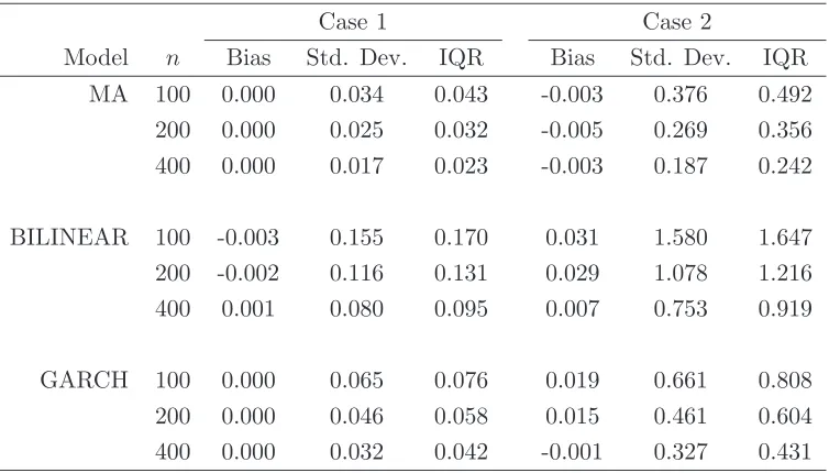
b= 0.5; (GARCH) ω= 0.1,α= 0.1, andβ = 0.8. We set T _{∈ {}100,200,400_}.

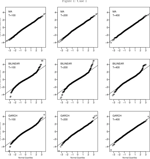
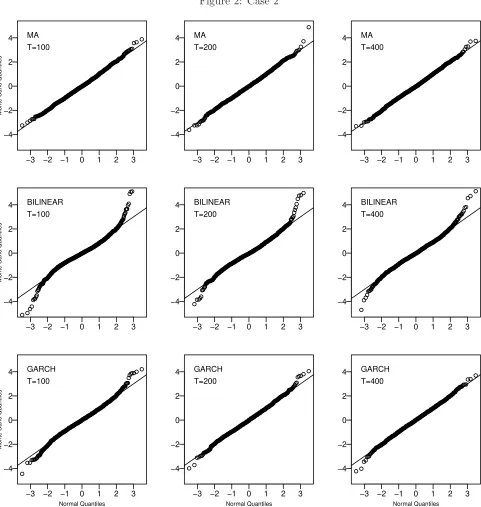
As for Theorem 3.1, we set h(x, y) = xy and J(u) = φ(u), where φ(·) represents the probability density function of a standard normal random variable. We call this Case 1 and it is such thatT_{(F) = 0.} Similarly, for Theorem3.2, we setJ(u) = 1 and choosekin (3.7) by standard cross-validation, see e.g. Hart and Vieu(1990). This is called Case 2 andθ0 in (1.3) equals 0 as well.

also included. For the (MA) process, the asymptotic normal approximation is very accurate for all sample sizes and in all cases. For the nonlinear processes (BILINEAR) and (GARCH) the normal approximation at the tails is better for a sample size of 400 than it is for 100 observations. In all models, as suggested by our results, the small sample tail behavior of the estimators becomes closer to that of a normal as the sample sizes increases.

From the results of Table 1, one observes that the proposed estimators work very well in terms of Monte Carlo bias (Bias), standard deviation (Std. Dev.) and inter-quartile range (IQR). In general, the proposed estimator of T_{(F) = 0 in Case 1 is generally unbiased for the (MA) and (GARCH)} processes, and in Case 2, the bias tends to decrease with the sample size quite rapidly. In all the cases, as predicted by Theorems 3.1 and 3.2, the simulated standard deviations and inter-quartile ranges decrease when the sample size increases.

4.2 Empirical Example: Consumer Surplus Estimation

In a classic paper, Engle et al. (1986) used a partial linear model to study the impact of weather and other variables on electricity demand. Since fully nonparametric models are becoming popular in Economics, see e.g. Huynh and Jacho-Ch´avez (2009), we use this framework to illustrate the utility of our estimator by applying our methodology to estimate consumer surpluses based on a fully nonparametrically estimated demand function for electricity in the Canadian province of Ontario. In particular, we calculate monetary gains obtained by consumers when facing lower prices than the one they are willing to pay - this is known as consumer surplus in Economics.

The data for this analysis come from the Ontario Hydro Corporation and is made publicly available by Yatchew (2003). The data consist of 288 quarterly observations in Ontario for the period 1971 to 1994 of the following variables: elect - log of monthly electricity sales in millions of Canadian dollars,

tempt - heating and cooling degree days relative to 68◦F, relpricet - log of ratio of price of electricity

to the price of natural gas, and gdpt - log of Ontario gross domestic product in millions of Canadian

dollars. Notice that tempt is the difference between the number of days the temperature is below 68◦F

(20◦C or room temperature) and number of days the temperature is above 68◦F. If the net cooling days is negative it implies that the monthly temperature is colder than 68◦F while positive is that it is positive (more hotter) days.

We setYt:= elect−gdpt - this normalization is suggested byYatchew (2003, Chapter 4) to enforce

a cointegration relationship, and Xt:= [tempt,relpricet] in (1.3). We then estimate a version of θ0 at

different levels of tempt. In particular, our calculation asks what would happen if the relative prices of

electricity versus natural gas in 1994 (fourth quarter) were set to 1989 prices (fourth quarter). During that period, electricity prices increased by 22.6 percent while gas increased by 9.2 percent for a net increase of 13.4 percent. For illustrative purposes, we compute the consumer surplus for the three levels of tempt: 1) median cold month (-397), 2) zero, and 3) median hot month (94). Our estimates

utilize k= [83,2] found via cross-validation as suggested by Hart and Vieu(1990). Overall, the largest consumer surplus gain is for cold months with 62.7 million normalized dollars. When tempt tends to

million. Overall, these estimates are reasonable, since consumer surplus gains are expected to be higher for households when the temperature is extremely cold or hot.

Acknowledgements

We would like to thank the Editor, Associate Editor and two anonymous referees for many helpful comments and suggestions. We also thank Juan Carlos Escanciano, Ingrid Van Keilegom, and Lanh Tran for their insightful and useful comments and suggestions in earlier drafts of this paper. We acknowledge the usage of the ‘np’ package byHayfield and Racine(2008), and the assistance of Takuya Noguchi in implementing the Monte Carlo experiments in the Quarry High Performance Clusters at Indiana University. We gratefully acknowledge support by the Social Sciences and Humanities Research Council of Canada grant (SSHRC Grant 410-2011-1700). The views expressed in this article are those of the authors. No responsibility for them should be attributed to the Bank of Canada. All remaining errors are the responsibility of the authors.

5

Proofs of Theorems

For brevity the proofs of the theorems are presented in concise format while all auxiliary results are available in Appendix A. Similarly, Appendix B restates various known results in the literature that are used in our proofs for the paper to be self-contained. The notation ‘Const.’ refers to any generic positive constant that may take different values for each appearance.

5.1 Proof of Theorem 3.1

The proof proceeds in three steps:

Step 1: Let Fǫ(·|I) = F(·|I) +ǫ(FT −F(·|I)) denote a ǫ-perturbation of F(·|I) in the direction

(FT −F(·|I)). Then,

φ(ǫ) =T_{(Fǫ) =} Z

RN+1

J(Fǫ(y))h(x, y)dFǫ(x, y).

Since the Gˆateau derivative of T_{(Fǫ) in the direction FT −F is defined as the right derivative of φ(ǫ)} at 0, we obtain

T′_{(FT −F(·|I)) =φ}′₍₀+_), =

Z

RN+1{

FT(y)−F(y|I)}J

′

(F(y|I))h(x, y)dF(x, y|I) + Z

RN+1

J(F(y|I))h(x, y)d{FT(x, y)−F(x, y|I)}

= Z

RN+1{

FT(y)−F(y|I)}J

′

(F(y|I))h(x, y)f(x|Y =y,I)f(y|I)dxdy

+ Z

RN+1

J(F(y|I))h(x, y)d{FT(x, y)−F(x, y|I)},

= Z

R{

FT(y)−F(y|I)}J

′

(F(y_|I))mh(y;I)dF(y|I) +

Z

RN+1

J(F(y_|I))h(x, y)d_{FT(x, y)−F(x, y|I)},

= Z

R{

FT(y)−F(y|I)}mh(y;I)dJ(F(y|I)) +

Z

RN+1

wheremh(y;I) =E[h(X, Y)|Y =y,I]. Integration by parts yieldsRR{FT(y)−F(y|I)}mh(y;I)dJ(F(y|I)) =

−RRJ(F(y|I))mh(y;I)d{FT(y)−F(y|I)} − R

RJ(F(y|I)){FT(y)−F(y|I)}dmh(y|I). It follows that T′_{(FT −F(·|I)) =}

Z

RN+1

J(F(y_|I))h(x, y)dFT(x, y)−

Z

R

J(F(y_|I))mh(y;I)dFT(y)

−

Z

R

J(F(y|I)){FT(y)−F(y|I)}dmh(y|I),

= 1

T

( _T X

t=1

J(F(Yt|I)){h(Xt, Yt)−mh(Yt|I)}

−

T

X

t=1

Z

R

J(F(y_|I))_{I_{(Yt ≤y)−F(y|I)}dmh(y|I)}

)

.

Hence, by the Taylor formula: φ(1) =φ(0) +Pℓ_k−₌₁1 k!−1φ(k)(u)_u=0+ +ℓ!−1φ(ℓ−1)(v), wherev∈[0,1], we obtain:

T_(FT)−T_{(F(·|I)) =}T′_{(FT −F(·|I)) +RT, (5.1)} whereRT is the remainder of the above expansion.

Step 2: We are now ready to prove the weak convergence ofT′_{(FT −F(·|I)). An application of the} martingale approximation for the processPT₁ Wtyields

T

X

1

Wt= T

X

1

W_t∗+fW1−WfT+1, (5.2)

where W_t∗ is defined from Lemma A.4; and Wft = P∞s=1E[Ws|Ft−1]. The asymptotic behavior of

T−1/2PT

1 Wtis determined by those of two terms, T−1/2

PT

1 Wt∗ and T−1/2(fW1−WfT+1).

To derive the asymptotic behavior of T−1/2P₁TW_t∗, note that W_t∗ is a martingale difference se-quence. Thus a Central Limit Theorem for martingale difference sequences (see e.g.Chow and Teicher, 1978, p. 336) can be applied; and the variance of the above sum is just EW₁∗2_|I given in Lemma

A.4.

Under Assumptions A1,A2 and A3a, the variance E[W₁∗2_|I] can easily be derived by sequentially applying LemmasA.2-A.4. To finish with deriving the asymptotic normality ofT−1/2PT₁ W_t∗, we need to check the Lindeberg condition: For an arbitrarily small constant, δ, it follows that

1

T

T

X

1

E

E

W_t∗21(W_√t∗

T > δ)

Ft−1 I

=E[W_t∗21(W_t∗> δ√T)_|I],

≤ kW₀2_kp,IP(Wt∗ ≥δ

√

T_|I)=p_⇒0,

where the last inequality follows from H¨older’s inequality; and the limit in probability follows from the Tchebyshev inequality and AssumptionsA2aand A3a. Hence, we obtain

1

√

T

T

X

1

To derive the asymptotic behavior of T−1/2(fW1−fWT+1), note that Wtis Ft-measurable. Given some

generic constant, δ >0, under Assumptions A2and A3awe obtain

P

f

W1−WfT+1 √

T

≥δ

!

≤2P |√fW1|

T ≥ δ

2 !

≤ kfW1kp

δ√T −→0 as T −→ ∞. (5.4)

From Eqs. (5.3) and (5.4), we obtain

√

TT′_{(FT −F(·|I))=}W_{⇒N(0, σW}2 _{). (5.5)}

Step 3: We conclude the proof by studying the limiting behavior of the remainder term,_RT, from the

Gˆateau expansion, i.e.

RT =

Z

RN+1

h(x, y)_{J(FT(y))−J(F(y|I))}dFT(x, y) +

Z

R

mh(y;I)d{K(FT(y))−K(F(y|I))}

+ Z

R

J(F(y_|I))_{FT(y)−F(y|I)}dmh(y|I),

whereK(u) =R₀uJ(v)dv. Some basic algebra yield

RT

= Z

RN+1

h(x, y)

J(FT(y))−J(F(y|I))

FT(y)−F(y|I) −

J′(F(y|I))

{FT(y)−F(y|I)}dFT(x, y)

−

Z

R

K(FT(y))−K(F(y|I))

FT(y)−F(y|I) −

J(F(y|I))

{FT(y)−F(y|I)}dmh(y|I)

−

Z

R

J(FT(y))−J(F(y|I))

FT(y)−F(y|I) −

J′(F(y_|I))

{FT(y)−F(y|I)}mh(y;I)dFT(y)

+ Z

RN+1

J′(F(y_|I))_{FT(y)−F(y|I)}h(x, y)dFT(x, y)

−

Z

R

J′(F(y|I)){FT(y)−F(y|I)}mh(y;I)dFT(y)

,

= _{Ra− Rb− Rc}+_Rd,

where the definitions of _Ra,_Rb,_Rc and _Rd should be apparent. We now bound each term in the last equality as follows:

Terms _Ra,_Rb,_Rc: Using an absolute value inequality, we have

√

TRa ≤ sup

1≤t≤T

√

T|FT(Yt)−F(Yt|I)|

× sup

1≤t≤T

J(F_FT_T(Y_(Yt))_t)−−_FJ(₍F_Yt(_|IYt₎|I))−J ′

(F(Yt|I))

_T1

T

X

t=1

|h(Xt, Yt)|.

The Birkhoff-Khintchine theorem (see e.g.Varadhan,2001, p. 132) yields, under AssumptionA1,

1

T

T

X

t=1

|h(Xt, Yt)|=⇒E[|h(Xt, Yt)|

Moreover, by the same arguments used in the proof of Step 2, we can prove that Assumption A2b

implies that limT−→∞supy∈R PT

s=1kP(Ys≤y|FY0)−P(Ys ≤y|I)kp/(p−1)<∞. Hence, it immediately follows that sup_1≤t≤T√T|FT(Yt)−F(Yt|I)|=Op(1) by Skorokhod representation theorem. Since the

Birkhoff-Khintchine theorem implies that _|FT(Yt)−F(Yt|I)| = oa.s.(1) for every t ∈ {1, . . . , T}, an

application of the stochastic mean-value theorem (see, e.g., White and Domowitz(1984)) yields

sup

1≤t≤T

J(FT(Yt))−J(F(Yt|I))

FT(Yt)−F(Yt|I) −

J′(F(Yt|I))

=oa.s.(1).

Therefore, we obtain √T_Ra = op(1). Using a similar argument and the Lebesgue dominated

conver-gence theorem, we can verify that √TRb =op(1) and

√

TRc=op(1).

Term _Rd: Firstly, notice that

E[√T_Rd2] =EhJ′2(F(Yt|I)){FT(Yt)−F(Yt|I)}2{h(Xt, Yt)−mh(Yt|I)}2

i

+ 1

T

T

X

t=1

s=1

t6=s

EhJ′(F(Yt|I))J

′

(F(Ys|I)){FT(Yt)−F(Yt|I)}{FT(Ys)−F(Ys|I)}

× {h(Xt, Yt)−mh(Yt|I)}{h(Xs, Ys)−mh(Ys|I)}] =Rd;1+Rd;2.

Using the fact that J′(F) is bounded and H¨older’s inequality, we obtain

Rd;1 ≤ Const._×{FT(Yt)−F(Yt|I)}2

p/(p−1)

_{h(Xt, Yt)−mh(Yt|I)}2

p. In view of the

Birkhoff-Khintchine theorem and the dominated convergence theorem, we obtain _{FT(Yt)−F(Yt|I)}2

p =

oa.s.(1). Hence, under AssumptionA1, we have

_{h(Xt, Yt)−mh(Yt|I)}2_p <∞.

Then,Rd;1=oa.s.(1).

In addition, we have

Rd;2 ≤ Const.× k{FT(Yt)−F(Yt|I)}k2_2p× T

X

τ=1

1₋ τ

T

kE[h(Xτ, Yτ)h(X0, Y0)|Fτ,Y,I]−mh(Yτ)mh(Y0)k_p/(p−1), where

k{FT(Yt)−F(Yt|I)}k22p =oa.s.(1). Thus, under Assumption A3b, we can deduce thatRd;2=o(1).

5.2 Proof of Corollary 3.1

Assumption B1 essentially implies Assumption A1. Assumption B2 implies Assumption A2a while Assumption A2b naturally follows from the ergodicity of the processes under study.

In light of Lemma A.5, Assumption B3a implies that P∞_t=1Kt(p) < ∞, where the term Kt(p)

inStep 1 in the proof of Theorem3.1, one needs AssumptionsA1andA3b. AssumptionA3b is verified as follows:

E[h(Xτ, Yτ)h(X0, Y0)|Fτ,Y]−mh(Yτ)mh(Y0)

=E

{h(X0, Y0)−mh(Y0)}E[h(Xτ, Yτ)−mh(Yτ)|F0,Fτ,Y]

Fτ,Y

≤ kh(X0, Y0)−mh(Y0)k_2,F0,Y Eh(Xτ, Yτ)−mh(Yτ)F0,X,F_τ,Y

2,Fτ,Y .

An application of H¨older’s inequality yields

kE[h(Xτ, Yτ) − mh(Yτ)

_F0,X,F_τ,Y

2,Fτ,Y

= Eheh1(ξτ◦−1|ξN+1,τ)|ξ◦0, ξN+1,τ

i

−Eheh1(ξ◦∗τ−1|ξN+1,τ)|ξ0◦, ξN+1,τi

2,Fτ,Y

≤ eh1(ξτ◦−1|ξN+1,τ)−eh1(ξ◦∗τ−1|ξN+1,τ)

2,Fτ,Y

= α∗_τ−1(ξN+1,τ),

whereξ◦∗_τ is ξ◦_τ with the whole past ξ₀◦ replaced by an i.i.d. copy ξ₀◦′. Another application of H¨older’s inequality yields

kE[h(Xτ, Yτ)h(X0, Y0)|Fτ,Y]−mh(Yτ)mh(Y0)k_p/(p−1) ≤ kh(X0, Y0)−mh(Y0)k2,F0,Y

p/(p−1)

α∗_τ−1(ξN+1,τ)

p/(p−1).

Hence, it immediately follows that P∞_τ=1α_τ∗₋₁(ξN+1,τ)

p/(p−1) <∞ implies AssumptionA3b.

5.3 Proof of Theorem 3.2

Some algebra yields the following expansion:

√

T(bθ₋θ0) = √1

T

T

X

t=1

J(t/T)Y(t)−g(X[t])

f(X_[t])

+ √1

T

T

X

t=1

J(t/T) Y(t)−g(X[t])

(

T_L(V1)RNT(X[t], k)

k −

1

f(X_[t]) )

+ √T

( _T X

t=1

J(t/T)L(V1)g(X[t])R

N

T(X[t], k)

k −

Z

X

g(x)dx

)

,

= _T1T +T2T +T3T,

where the definitions of _TlT (l = 1,2,3) should be apparent. These three components are analyzed in

each of the following 3 steps:

Step 1: Since AssumptionsC2,C3b,C4a, andC4bimply AssumptionsA1,A2, andA3. An application of Theorem 3.1yields

The proof concludes by showing that _T2T =op(1) andT3T =op(1).

Step 2: Since E[Y(t)−g(X[t])|FT,X] = 0, we can show that

E[_T2T] =

1

√

T

T

X

t=1

J(t/T)E

"

Y_(t)−g(X_[t]) (

T_L(V1)R_TN(X[t], kT)

kT −

1

f(X_[t]) )#

= E

"(

TL(V1)R_TN(X[t], kT)

kT −

1

f(X_[t]) )

E[Y_(t)−g(X_[t])_|FT,X]

# 1

√

T

T

X

t=1

J(t/T) = 0.

Furthermore,

E[_T22_T] = 1

T

T

X

t=1

J2(t/T)E



_{Y_(t)−g(X_[t])_}2 (

TL(V1)RTN(X[t], kT)

kT −

1

f(X_[t]) )2



+ 1

T

T

X

s=1

t=1

s6=t

J(t/T)J(s/T)EY_(t)−g(X_[t]) Y_(s)−g(X_[s])

×

(

TL(V1)R_TN(X[t], kT)

kT −

1

f(X_[t]) ) (

TL(V1)R_TN(X[s], kT)

kT −

1

f(X_[s]) )#

= _T2T;1+T2T;2.

Using the Cauchy–Schwarz inequality and the fact that the score function J(·) is bounded, we have

T2T;1 ≤ Const.×

_{Yt−g(Xt)}2

2

_T

L(V1)RN_T(Xt, kT)

kT −

1

f(Xt)

2

2

,

and, by virtue of the stationarity of _{Xt, Yt},

T2T;2 ≤ Const.

×_T1

T

X

s=1

t=1

s6=t

TL(V1)RNT(Xt, kT)

kT −

1

f(Xt)

TL(V1)RNT(Xs, kT)

kT −

1

f(Xs)

p

≤ Const._× sup

1≤t≤T

TL(V1)RNT(Xt, kT)

kT −

1

f(Xt)

TL(V1)RTN(Xs, kT)

kT −

1

f(Xs)

p

×_T1

T

X

s=1

t=1

s6=t

kE[YtYs|Xt,Xs]−g(Xt)g(Xs)kp/(p−1)

= Const.× sup

1≤t≤T

TL(V1)RNT(Xt, kT)

kT −

1

f(Xt)

TL(V1)RTN(Xs, kT)

kT −

1

f(Xs)

p ×2 T X τ=1 1− τ

T

kE[YτY0|Fτ,X]−g(X_τ)g(X₀)k

p/(p−1)

≤ Const._× sup

1≤t≤T

T_L(V1)RNT(Xt, kT)

kT −

1

f(Xt)

T_L(V1)RTN(Xs, kT)

kT −

1

f(Xs)

p × T X τ=1

kE[YτY0|Fτ,X]−g(X_τ)g(X₀)k_p/(p

−1)

Under Assumption C2b, we have _kYt−g(Xt)k4 ≤ kYk4 <∞. Moreover, under Assumptions C3 and

C7, LemmaA.6 and the dominated convergence theorem yield

lim T−→∞

T_L(V1)RNT(Xt, kT)

kT −

1

f(X_t) 2

2

= 0.

Hence, we have _T2T;1 −→ 0. By the same argument, we can show that, under Assumption C4c, T2T;2 −→0. Therefore, it follows thatT2T =op(1).

Step 3: Notice that

T3T =

1 √ T T X t=1

{J(1/T)₋1_}g(X[t]) b

f(X_[t]) + 1 √ T T X t=1

g(Xt)

b

f(Xt)

−√T

Z

X

g(x)dx

= _T3T;1+T3T;2,

wherefb(x) =kT/TL(V1)RNT(x, kT) as previously defined. We start with the first term T3T;1 equals

1 √ T T X t=1

{J(t/T)−1}g(X[t])

( 1 b

f(X_[t])− 1

f(X_[t]) )

+ √1

T

T

X

t=1

{J(t/T)−1}g(X[t])

f(X_[t]) = T3T;1a+T3T;1b.

0< pi ≤ ∞and 1/r=Pki=11/pi, thenkQik=1uikr≤Qik=1kuikpi, yields

E[|T3T;1a|2]≤

1

T

T

X

t=1

{J(t/T)−1}2E

 g2(Xt)

1 b

f(Xt)

− 1

f(Xt)

2 

+ 21

T

T

X

t=1

s=1

t6=s

|{J(t/T)₋1_}{J(s/T)₋1_}|E

"

g(X_[t])g(X_[s]) 1 b

f(X[t])

− 1

f(X_[t]) 1 b

f(X[s])

− 1

f(X_[s]) #

≤ kg2(X0)k2

1 b

f(Xt)

− 1

f(Xt)

2 2 1 T T X t=1

{J(t/T)−1}2

+ 2_kg(X0)k24

1 b

f(Xt)

− 1

f(Xt)

2 4 1

T|J(0)−1|

T

X

τ=1

|J(τ /T)₋1_|.

Under Assumptions C3 and C7, Lemma A.6 holds. The score function J(_·) is bounded. Assumption

C2b implies that E[g4_(X

0)] < ∞. It then follows that limT−→∞E[|T3T;1a|2] = 0. With the same

argument, we can also show that limT−→∞E[|T3T;1b|2] = 0. Hence, we obtain

T3T;1=op(1). (5.6)

Step 3: To finish the present proof, we need to show that_T3T;2=op(1). Suppose that the distribution

functionF(x) is invertible (i.e., given somex_{∈ X} there exists a realization of the Uniform[0,1] random variable, U, such that x=F−1(u), where F−1(u) is the inverse cdf). In view of Lemma B.5 and the definition of integrals along a curve in RN _{(or line integrals), see e.g. Apostol (1969, Definition 10.1),}

one can derive the following approximation:

E

g(X)

f(X)

= Z

X

g(x)

f(x)dF(x) = Z

[0,1]

g F−1_(u)

f(F−1_(u))du=

2N

X

s=0

Z (s+1)2−N

s2−N

g F−1_(u)

f(F−1_(u))du

≈ 2−N

2N

X

s=0

g F−1(us)

f(F−1_(u

s))

,

where us ∈ [s2−N,(s+ 1)2−N). Without any loss of generality let us choose N = log2T. It then

follows that:

T3T;2 =

1 √ T T X t=1 (

g(Xt)

b

f(Xt)

− g(F−

1_(u

t))

f(F−1_(u

t))

)

+op(1).

Recalling Assumption C5a, the set _X is closed and bounded. As T becomes sufficiently large, it is possible to find a ρ₋ball of radius δN(T) =ǫ2−N(T), which centers at τt such that F−1(ut) ∈BδN(τt),

where N_{(T) increases with T, thus implicitly depends on T, though in what follows we will suppress} the dependence ofN _{onT unless confusion is likely. Hence, we have}

T3T;2 =

1 √ T T X t=1 (

g(Xt)

b

f(Xt)

− g(Xτt)

f(Xτt) )

+ √1

T

T

X

t=1

g(Xτt)

f(Xτt)

− g(F−

1_(u

t))

f(F−1_(u

t))