ELECTROMAGNETIC IMAGING METHOD BASED ON TIME REVERSAL PROCESSING APPLIED TO
THROUGH-THE-WALL TARGET LOCALIZATION
N. Maaref, P. Millot, and X. Ferri`eres
ONERA - DEMR
2 Avenue Edouard Belin, 31055 Toulouse, France
C. Pichot
LEAT - CNRS
250 rue Albert Einstein, 06560 Valbonne, France
O. Picon
Universit`e Paris-Est, ESYCOM, EA2552 5, Bd Descartes, 77454 Marne-la-Vall`ee, France
Abstract—A time reversal method is studied and adapted to through-the-wall detection and localization of moving targets. Tests are realised on experimental data in a synthetic aperture radar configuration. The efficiency of the method to extract a moving target from a cluttered environment is proved on experimental data.
1. INTRODUCTION
60 Maaref et al.
particular, experimental measurements are performed in a spotlight synthetic aperture radar configuration [5, 6] and then are treated by a signal processing method to obtain an image of the scene. In this radar configuration, an antenna array is used on reception and a fixed one on emission. Many signal processing methods can be considered for target localization. We have chosen to focus on an emerging method in electromagnetic detection field, especially in a cluttered environment [7]: time-reversal adapted here to through-the-wall localization. In this work, in particular, time reversal processing is applied to experimental data to demonstrate the localization of dielectric moving objects behind a 10 cm thick brick wall.
2. TIME REVERSAL METHOD
Time reversal is a method that has proved its efficiency in recent years especially in acoustics [8, 9] but also in UWB communications [10– 12]. This method is based on the reciprocity of Maxwell’s equations in a time-invariant medium. It can be used to localize a source of energy in space. In fact, we assume that we have a pulsed UWB source. This emitted signal is recorded by an array of receivers. It has been proved [13] that by reversing in time this data and radiating it from the same array, we focus on the source location. The focusing precision is imposed by the size of the array of transceivers and may even increase in presence of multipaths [14]. In this particular case, there is a source radiating a plane wave. This field is scattered by a collection of targets and the environment which can be considered as secondary sources in the time-reversal processing. Fields are recorded, time reversed and re-radiated from receivers. This last step is achieved computationally. In the observed scene, focusing occurs on all scattering points (target + clutter). However, if we assume that background is stationary so its signature (without the target) may be measured and subtracted to the whole signature (target + clutter). This new signal is then backscattered from receivers into medium. Now focusing only occurs on the target.
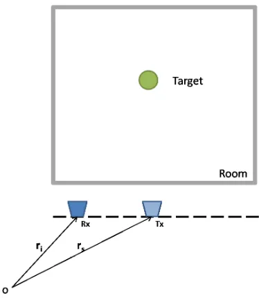
Let us consider a single target located in a time-invariant clutter. The single source is located at rs and the N positions of the receiving
antenna are denoted as ri (1 ≤ i ≤ N) (see Fig. 1). Here, all
the possible interactions between the environment and the target are neglected. When the source emits a pulse of spectrum P(w), the incident field on the target point located atrc is given by:
E(rc, w) =P(w)G(rc, rs, w) (1)
Figure 1. Schematic of through-the-wall time-reversal imaging. The target is located in a room. Sensors are outside.
receiver positioni, the scattered field observed is: E(ri, w) = R(rc)E(rc, w)G(ri, rc, w)
= R(rc)P(w)G(rc, rs, w)G(ri, rc, w) (2)
whereR(rc) is the reflexion coefficient. It is important to note that in
62 Maaref et al.
η(r) is evaluated at each point of the domain:
η(r) =
w N
i=1
E∗(ri, w)G(r, ri, w)P(w)G(rs, r, w)
=
w N
i=1
[R(rc)P(w)G(rc, rs, w)G(ri, rc, w)]∗
G(r, ri, w)P(w)G(rs, r, w) (3)
In this equation, the first group of terms E∗(ri, w)G(r, ri, w)
corresponds to a classical time reversal process in which the recorded signals are phase conjugated and then re-radiated into the scene. The second group of termsP(w)G(rs, r, w) corresponds to a compensation
of the fact that the recorded signals don’t come from the target it self but are scattered by it. Due to the reciprocity theorem, we have: G(rc, rs, w) = G(rs, rc, w) and G(ri, rc, w) = G(rc, ri, w), thus
we obtain, on the equation (3), constructive interferences at r = rc.
The variation ofη(r) gives a 2D or 3D image which is a representation of the reflexion coefficient at each point of the scene. It is important to note that, in our case, the calculation of Green’s function is performed considering the free-space form and then a supplementary delay due to the propagation on the wall is introduced. The exact calculation of Green’s function was done numerically by a finite difference time domain (FDTD) method. Results obtained on our measurements are quite the same probably because of the nature of the wall and the range of frequencies used in this particular case. However, in a more complex medium, the exact calculation of Green’s function could become necessary.
3. EXPERIMENTAL SET UP
The experimental set up consists of a vector network analyser and of two ultra-wideband ETSA (exponentially tapered slot antenna) antennas (a transmitter and a receiver). This type of antennas has improved bandwidth and radiation characteristics [15].
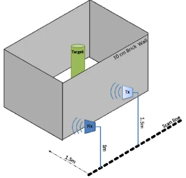
The receiving antenna is placed on a moving rail to synthesize an array on reception. Synthetic aperture radar configuration is chosen to improve the crossrange resolution. The size of the array is 1.8 meters and 18 positions are taken with an increment of 10 cm. Receiving antenna is elevated at about 1.2 meters above ground.
Figure 2. Experimental configuration.
Figure 3. Impulse response at each receiver position for a target placed at (1 m, 3.4 m).
by the attenuation of electromagnetic waves through walls. Fig. 2 shows this experimental configuration.
64 Maaref et al.
the array of receivers. These measurements are then computationally processed by time reversal method to give an image of the scene. Fig. 3 is a time domain representation of the signals measured at each antenna position when only one target is in the room (environment has been subtracted from the measurements).
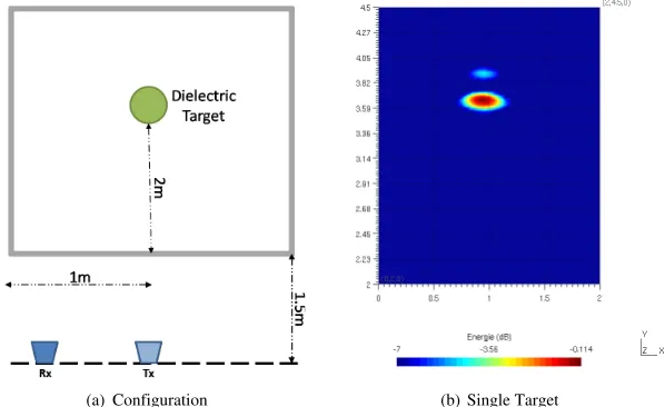
Figure 4. Localization of a single target.
4. RESULTS
Configuration
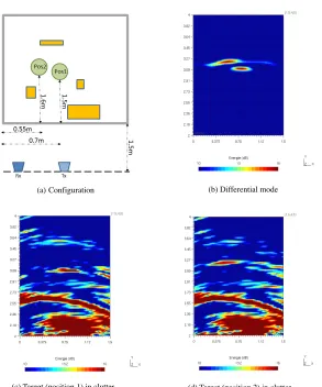
(a) (b) Differential mode
(c) Target (position 1) in clutter (d) Target (position 2) in clutter
Figure 5. Localization of a moving target in a cluttered environment.
been removed. This result shows the efficiency of our time-reversed imaging processing in the case of through-the-wall localization of a moving target even in presence of clutter.
5. CONCLUSION
66 Maaref et al.
has been performed. Moreover, we notice that, in order to track a target in a room, it is not necessary to perform a first calculation of the environment without the target. Taken advantage from the fact that the human target is necessarily moving, the differential mode would be sufficient. A future challenge would consist in being able to detect a very small movement in a more complex environment (concrete walls,numerous walls, multiple targets . . . ).
ACKNOWLEDGMENT
The main part of this study has been supported by the DGA. REFERENCES
1. Ferris Jr., D. D. and N. C. Curris, “A survey of current technolo-gies for through-the-wall surveillance (TWS),”Proceedings SPIE, Vol. 3577, 62–72, Jan. 1999.
2. Ahmad, F. and M. Amin, “A non coherent approach to through-the-wall radar imaging,” Proceedings of the 8th International Symposium on Signal Processing and Its Applications, Vol. 2, 28– 31, 2005.
3. Taylor, J. D.,Introduction to Ultra-wideband Radar Systems, C RC Press, 1995.
4. Chen, F. C. and W. C. Chew, “Time-domain ultra-wideband microwave imaging radar system,” Journal of Electromagnetic Waves and Applications, Vol. 17, No. 2, 313–331, 2003.
5. Soumekh, M., Synthetic Aperture Radar Signal Processing, John Wiley and Sons, Inc., New York, NY, 1999.
6. Chan, Y. K. and V. C Koo, “An introduction to synthetic aperture radar (SAR),” Progress In Electromagnetics Research B, Vol. 2, 27–60, 2008.
7. Liu, D., G. Kang, L. Li, Y. Chen, S. Vasudevan, W. Joines, Q. H. Liu, J. Krolik, and L. Carin, “Electromagnetic time-reversal imaging of a target in a cluttered environment,” IEEE Trans. on Antennas and Propagation, Vol. 53, No. 9, Sept. 2005.
8. Fink, M., “Time-reversal acoustics,”Physics Today, Vol. 50, No. 3, 34–40, 1997.
10. Xiao, S. Q., J. Chen, B.-Z. Wang, and X. F. Liu, “A numerical study on time-reversal electromagnetic wave for indoor ultra-wideband signal transmission,” Progress In Electromagnetics Research, PIER 77, 329–342, 2007.
11. Xiao, S., J. Chen, X. Liu, and B.-Z. Wang, “Spatial focusing characteristics of time reversal UWB pulse transmission with different antenna arrays,”Progress In Electromagnetics Research B, Vol. 2, 223–232, 2008.
12. Liu, X.-F., B.-Z. Wang, S. Xiao, and J. H. Deng, “Performance of impulse radio UWB communications based on time reversal technique,”Progress In Electromagnetics Research, PIER 79, 401– 413, 2008.
13. Lerosey, G., J. de Rosny, and A. Tourin, et al., “Time reversal of electromagnetic waves,” Phys. Rev. Lett., Vol. 92, No. 19, 2004. 14. Sarabandi, K., I. Koh, and M. D. Casciato, “Demonstration of
time reversal methods in a multi-path environment,”Proceedings of IEEE AP-S Symposium, Vol. 4, 4436–4439, Jun. 2004.