Copyright1998 by the Genetics Society of America
Approximate Analysis of QTL-Environment Interaction with No Limits
on the Number of Environments
Abraham B. Korol, Yefim I. Ronin and Eviatar Nevo
Institute of Evolution, University of Haifa, Mount Carmel, Haifa 31905, Israel Manuscript received December 9, 1996
Accepted for publication December 31, 1997
ABSTRACT
An approach is presented here for quantitative trait loci (QTL) mapping analysis that allows for QTL 3 environment (E) interaction across multiple environments, without necessarily increasing the number of parameters. The main distinction of the proposed model is in the chosen way of approximation of the dependence of putative QTL effects on environmental states. We hypothesize that environmental dependence of a putative QTL effect can be represented as a function of environmental mean value of the trait. Such a description can be applied to take into account the effects of any cosegregating QTLs from other genomic regions that also may vary across environments. The conducted Monte-Carlo simulations and the example of barley multiple environments experiment demonstrate a high potential of the proposed approach for analyzing QTL3E interaction, although the results are only approximated by definition. However, this drawback is compensated by the possibility to utilize information from a potentially unlimited number of environments with a remarkable reduction in the number of parameters, as compared to previously proposed mapping models with QTL3E interactions.
D
IFFERENTIAL expression of a phenotypic trait environments provides a significant increase instatisti-by genotypes across environments, or genotype3 cal power of QTL detection and accuracy of the
esti-environment (G3E) interaction, is an old problem of mates of QTL position and effect (Jansenet al. 1995).
primary importance for quantitative genetics and its However, such an analysis is limited by situations where
applications in breeding, conservation biology, theory the environments can be obviously characterized by
of evolution, and human genetics (EberhardandRus- some parameters, like day length or
irrigation-fertiliza-sel1966;Falconer1981;ViaandLande1987;Tiret tion treatments, etc. [like the “fixed effects” model of
et al. 1993; WuandStettler1997). Recent successful analysis of variance (ANOVA)]. When these
characteris-attempts to dissect quantitative variation into Mendelian tics are not available, the application of the “general”
genes employing molecular markers (mapping quanti- QTL3E mapping model (see below) is accompanied
tative trait loci, or QTLs) have shifted the focus of G3 by a tremendous number of parameters involved in the
E interaction analysis from the genotype to gene level model that increase as a product of the identified QTLs
(e.g., Paterson et al. 1991;Hayeset al. 1993; Asins et
and the number of environments where the traits were
al. 1994; Sari-Gorla et al. 1997). For breeding
pur-measured. In such a case, one could think about a
“ran-poses, the primary concern is possible environmental dom effects” model so that the number of parameters
instability in manifestation of mapped QTLs that might for each QTL will include only main effect, the variance
become candidates for marker-assisted selection. To of QTL 3 E interaction, and QTL position. Although
evaluate stability of QTL effects in crop species, dozens this option seems very attractive, it has its own
draw-of immortal mapping populations have been developed backs, especially if we are going to deal with
environ-for trait scoring under various environmental condi- mental variation associated with different localities.
In-tions (Hayes1994).
deed, some (or many) localities may manifest quite
Several algorithms and computer packages have been repeatable differences from each other, justifying the
proposed to conduct QTL mapping, allowing for QTL3 “fixed model” approach (Baker1996). Moreover, the
E interaction effects (Hayes et al. 1993; Jansenet al.
information of geographically-specific QTL effects may
1995;TinkerandMather1995;Romagosaet al. 1996;
be of practical importance. In such a case, a fixed effects
Beavis andKeim 1996; Utz andMelchinger 1996).
model is, whenever possible, preferable over the
ran-In addition to testing the hypothesis of QTL3E
inter-dom effects model, because the latter hides the biologi-action, simultaneous treatment of data from multiple
cal (geographic) specificity of the QTL effect, compress-ing all the results to an estimate of variance. The major goal of this paper is to present an approach of QTL
Corresponding author: Abraham B. Korol, Institute of Evolution,
Uni-mapping analysis, allowing for QTL 3 E interaction
versity of Haifa, Mount Carmel, Haifa 31905, Israel.
E-mail: [email protected] across a large (in fact, unlimited) number of
ments, without the necessity for a corresponding increase technical features. These could strongly affect the
mani-in the number of parameters. The proposed model is festation of quantitative traits and the effects of QTL
especially relevant in situations of geographic variation of but are difficult to characterize quantitatively. As first
external conditions, where the fixed model approach is suggested by Eberhard andRussel (1966), we
advo-desirable but not easy to implement. cate that the measured trait values of the mapping
popu-lation (e.g., trait means) may serve as objective integral characteristics of the environmental state. Accordingly,
THE MODEL a larger number of traits should provide a better
“bioin-dication.” In the simplest form, one can approximate Approximated description of environmental
depen-the environmental dependence of depen-the effect of allele dence of QTL effect: The main distinction of the
pro-substitution at a QTL by a polynomial over the mean posed model is in the choice of approximation of the
values of the same trait across the environments. The dependence of putative QTL effects on environmental
following example of a QTL mapping in a barley experi-states. In reality, each environment is a complex of
abi-ment (Hayeset al. 1996) with measurements conducted
otic (temperature, humidity, ion concentration, etc.),
biotic (parasites, pathogens, competitors, etc.), and agro- in many environments, illustrates the idea (Figure 1).
Figure1.—Regression approximation of QTL substitution effect a as a function of mean trait valuem
i. Data on barley malting quality traits fromHayeset al. (1996). Circles represent pairs (ai,m
For some putative QTLs, the dependence on mean value Ui(x)5 pifqq(x)1 (12 pi)fQ Q(x), i51,4 , (2)
of the respective traits explains a large part of the
envi-where the proportionspi5 pi(r1,r2) are dependent on
ronmental variation of the QTL effect. This suggested
r1 and r2. Here, fqq(x) and fQ Q(x) are the trait density
approach does not exclude the possibility to take into
distributions in the QTL groups qq and Q Q, respectively. account any additional information, like temperature,
With no interference, p1 5 (1 2 r1)(1 2 r2)/(1 2 r);
day length, water regime, etc., that might characterize the
p25r1(12 r2)/r ;p35 12 p2; andp45 12 p1.
environments (e.g.,Jansen et al. 1995). These “physical”
In a single-environment formulation, one could test characteristics can be introduced into the model parallel
whether or not the observed variation of x is associated to the bioindicatory terms (e.g., polynomial over the mean
with segregation in interval Mk/mk2Mk11/mk11and
iden-values) together with terms characterizing the
depen-tify the corresponding locus Q/q. Provided recombina-dence of the putative QTL effect on interaction between
tion rate between marker loci is known, the vector of n1
the physical and bioindicatory factors. Another approach
parameters specifying the putative QTL can be presented
to analyze QTL 3E interaction without direct
specifica-asun15 {r ,m,a,s2}. The assumption of no association
be-tion of the physical characteristics of the environments
tween segregation in Mk/mk 2 Mk11/mk11 interval can
was recently proposed byRomagosaet al. (1996). Their
formally be presented by another set of parameters, algorithm is based on clustering the environments using
u 5 un0 5 {m,s2}. The null hypothesis {H
0: u 5 un0}, as
a few (e.g., two) detected QTL with most variable effects
contrasted with the alternative {H1: u 5 un1}, can be
across environments. Actually, this is a different version
investigated with the likelihood ratio test approach of the same general idea of bioindicators as a tool for
(Wilks1962). If H0is true, the statistic
characterizing “anonymous” environments.
Clearly, the results one could obtain by means of the x2(H
1vs. H0)5 2ln[maxL(un1)/maxL(un0)] (3)
method of QTL 3 E analysis proposed in this paper u
n1P S1 un0 PS0
will be approximate, allowing, at best, to consider the
is distributed asymptotically as chi-square with n12n0
major part of QTL 3 E interaction. However, as will
d.f., where S0 and S1 are the parameter spaces
corre-be demonstrated corre-below, the possibility to work with an
sponding to H0and H1, respectively (Wilks1962;Zeng
unlimited number of environments without increasing
1994). Thus, if x2 exceeds some critical value
corre-the number of parameters, as compared to usual
map-sponding to a preset level of significance a, the null
ping models with QTL 3 E interactions, may
signifi-hypothesis can be rejected. In such a case, numerical cantly offset loss-of-accuracy drawback, resulting in
in-values of the parameters that maximize L(un1) are
con-creased power to detect QTL 3 E interactions and in
sidered maximum likelihood estimates of the parame-improved accuracy of estimates of QTL genomic location.
ters characterizing Q/q, its effect and position (Weller
Mixture-model of interval QTL mapping: Consider
1986;LanderandBotstein1989; KnottandHaley
a simplified situation when the trait of interest (x)
de-1992). As applied to (3), the test statistic will have pends on a single QTL, Q/q. We will confine the analysis
n12n05 42 25 2 d.f.
to dihaploid mapping populations (which also applies
In multiple environments, we could use the foregoing to backcrosses and recombinant inbreds), but it can
to trait measurements obtained under several environ-easily be extended to other population structures. Then,
mental conditions. Namely, when comparing the fore-for an arbitrary genotype of the mapping population,
going alternatives H0and H1, QTL3 E interaction
ef-the trait measurement in ef-the ith environment can be
fects could be included in the model and tested against presented as
the alternative of no QTL 3 E interaction. In other
xi 5 mi10.5gai1ei, (1) words, an additional group of hypotheses {H
2:u 5 un2}
could be considered that assume a dependence of the
where miis the mean trait value in the ith environment,
target QTL effect and, possibly, of the residual variance,
g is either 11 (for QQ genotypes) or 21 (for qq
geno-on envirgeno-onment. Vector un2 of the full model,
corre-types), aiis the effect of allele substitution at putative QTL
sponding to H2 with environment-specific parameters
on trait in environment i, and eiis a random variable with
ai, s2
i, and mi will then contain 3p 1 1 components,
zero mean and variance s2
i. If we find ai z a for any i,
where p is the number of environments. Consequently,
then no G3E interaction is manifested by Q/q.
un1 specifying H1 (constant effect ai z a of the QTL
Assume that Q/q resides in some interval (k,k1 1) of
across environments, though allowing for variable s2
i
a chromosome marked by a series of marker loci, Mj/mj,
andmi) contains 2p12, whileun0(no QTL on the tested
with recombination rates r1 and r2 in Mk/mk2Q/q and
chromosome) contains 2p parameters.
Q/q 2 Mk11/mk11, respectively. For simplicity, we
con-In the simplified case of only one QTL segregating fined the analysis to the “no interference” case. For a
in the mapping population, no correlation between trait dihaploid (backcross) mapping population, the expected
measurements across environments are expected. With densities of the trait x in each of the four marker groups
this assumption, instead of the test statistics (3), one can
Umkmk11(x)5U1(x), UMkmk11(x)5 U2(x), UmkMk11(x)5U3(x),
with df 5 2p 1 2 2 2p 5 2. If H0 is rejected (ai ? Equation 3, a and b, we could replace the corresponding
0), then the obvious benefit of the corresponding multi- coordinates of the parameter vectorsuniby polynomials:
environmental model is the striking increase in the
num-ai5 a01 a1mi1 a2m2i 1. . .1 asmsi,
ber of measurements, resulting in higher precision of
s2
i 5 b01 b1mi1 b2m2i 1. . .btmti, i 51,p . (4)
parameter estimates (e.g.,Jansenet al. 1995). No less
im-portant is the possibility to conduct the following two tests: In other words, instead of estimates of r
1, ai, ands2i, the
procedure will provide ML-estimates of r1and regression
x2(H
2vs. H0)52ln[maxL(un2)/maxL(un0)] (3a)
coefficients a0, a1,..., as,b0, b1, and bt. The following
un2PS2 un0PS0
information about these coefficients will be useful. One
with df5 3p1 12 2p5p11, and can represent the approximation (4) in form of
devia-tions from the mean values of the traitmaveraged over
x2(H
2vs. H1)52ln[maxL(un2)/maxL(un1)] (3b)
environments, i.e., with terms ak(m 2 mi)kandbj(m 2
un2PS2 un1PS1 m
i)j, instead ofakmki andbjmji. Then, the genetic
interpre-tation of the coefficienta0is that it specifies the average
with df5 3p 11 2 (2p 1 2) 5p 2 1. Note that the
substitution effect at the putative QTL, whereas coeffi-same d.f. for the test statistics will be obtained if the
cientsai (i.0) reflect the stability of the QTL effect
entire analysis is conducted for the centered data, so
over environments. This parallels the stability analysis
thatmiare subtracted from the individual measurements
of Eberhardand Russel (1966), although they used
at corresponding environments.
only linear regression in their model. There are differ-The asymptotic distribution of the test statistics (3)
ent reasons why linear approximation for QTL depen-in the multi-depen-interval mappdepen-ing remadepen-ins unknown (see
dence on environment may be not sufficient. For
exam-Zeng1994), but one could use extensive Monte-Carlo
ple, one may mention the effect of canalization of gene simulations in order to obtain an empirical critical value
effects (Gilbert1961;Rendel1967;Korolet al. 1981,
of the statistics for each considered situation. Our
previ-1994). Likewise, the coefficientb0specifies the residual
ous simulation studies (Korolet al. 1995) have shown
variance under average conditions, whereas bi (i.0)
that the chi-square distribution is a good approximation
reflect the stability of the residual variance with devia-for the test statistic (3), and here we will demonstrate
tion from average conditions. The changes in the resid-that it may also be suitable for the test statistic (3b).
ual variance may result from either QTL3E interaction
Regression specification of QTL 3 E interaction:
at other sections of the genome not accounted by the Ignoring possible variation of the QTL effect among
model or dependence of nongenetic components of environments may lead to erroneous breeding decisions
residual variation on environment. in subsequent applications of the mapping results, an
The degrees of polynomials in Equation 4 cannot be accompanied reduction in the power, and loss of
preci-predetermined before the mapping analysis. By con-sion in estimated QTL effects and genome location. On
trast, the analysis includes model adjustment with a
se-the contrary, accounting for QTL3 E interaction in
ries of polynomials a(m)5Pas(m) ands2(m)5P
s2 t(m),
the data obtained in multiple environments can strongly
and the final degrees s and t are to be chosen on the increase the resolution of the mapping experiment
basis of maximum statistical significance of the hypothe-(Jansenet al. 1995;TinkerandMather 1995).
How-sis QTL 3 E interaction vs. the alternative of no
ever, this proficiency is seriously attenuated by the
neces-QTL3 E interaction (see further analysis).
sity to build into the mapping model a large number
An important point of concern with the proposed of parameters specifying the working hypothesis of the
approach is how to proceed in a situation where the QTL effects. For example, an experiment with 10
envi-employed model allowed us to detect a significant QTL ronments will require a model with 31 parameters when
effect, but QTL3E interaction was not detected. Does
evaluating a single interval.
it mean that no QTL3E interaction is characteristic of
According to the proposed approach, the unknown
the revealed QTL or, alternatively, that this interaction
effects aiand, if desirable, the residual variancess2i are
exists, but the chosen parametrization (e.g., regression represented by low degree polynomials. For instance,
of QTL effects on mean trait values across
environ-with a cubic approximation for ai and a quadratic for
ments) poorly approximates the real dependence of the
s2
i, we will only need seven parameters instead of 20!
QTL effect on environment. One of the possible ways Clearly, the main question remains to what extent the
to overcome this obstacle will be presented below. bioindicating trait, or a (linear) combination of traits,
Obtaining parameter estimates: Maximum likelihood will indeed be informative with respect to the
depen-estimates of all of the parameters, includinga andb,
dence of the target QTL effect on environmental states.
are obtained using the procedure of numerical multipa-No prior answer is possible, but the foregoing examples
rameter optimization of functions L(u) from Equation
on barley (see Figure 1) demonstrate that such an
as-3, a and b. Optimization was by modified gradient method sumption is quite realistic, even with the simplest
univar-(Himmelblau1972). The possibility of multiple
max-iate mode of the approximation, ai 5 f(mi). Thus, in
RESULTS The results presented in Table 2 show that adequate
approximation of a(m) results in an appreciable
in-The efficiency of the proposed method was tested
crease in the power of both tests: H1vs. H0 (presence
through Monte-Carlo simulations. Three groups of
situ-of a QTL, allowing for ai5const ands2i ?const), and
ations were simulated: a single QTL (situations S1–S3),
H2 vs. H1 (presence of QTL3 E interaction, allowing
two unlinked QTLs (situations S4–S5), and several
un-fors2
i?const). Utilization of a(m) ands(m) polynomial
linked QTLs (situation S6) (Table 1).
approximations resulted in an improved precision in Single QTL: In the situation with a single QTL, no
the estimated QTL position (compare the estimated “between-environment” correlation is expected for the
position L and its standard error sL for MA and MG
residual (within QTL groups) variation. Thus, the
log-in Table 2). In situation S1 with the smallest average
likelihood functions 3a and 3b for the mixture model
simulated QTL effect, the power to detect the QTL at 3a and 3b could be calculated by summing up over all
the significance level of 1% was 45 and 34% for MA and environments and employing the polynomials of
Equa-MG, respectively, whereas the corresponding figures for tion 4. This assumes implicitly that after removing the
detection of QTL 3 E interaction were 41 and 29%.
effects of the QTL under consideration, the residuals
Note that this increased resolution of the MA model as are independent across environments. Clearly, such an
compared to the MG model was obtained using only idealization is correct if all residual genetic variation of
eight parameters (less than half of that in MG). Hence, the quantitative trait is taken into account by markers
the superiority of the MA model over MG is reflected
of other genomic regions, such as cofactors (Jansen
in the values of AIC. Likewise, the polynomial model
andStam1994;Zeng1994). This may not be the case,
providedz1.5–2-fold reduction in the estimated
confi-calling into question the applicability of the proposed
dence interval for the aiestimates across environments
approach to real data analysis. It is indeed a very serious
(Figure 2). problem, but as shown in the following section, the
With simulated data, it is easy to compare “the ade-conclusions may be fairly promising.
quate” and “nonadequate” approximations simply be-As a first step in demonstrating the idea of our
cause we know the employed model. The results in method, we here consider the simplest case of a single
Table 3 illustrate this point. As one can see, the adequate QTL. The dependence of the simulated QTL effect and
model (MA3) gave the highest power of detection of
the residual variance on environment was modeled as
both the presence of the QTL in question and QTL3
cubic and quadratic functions, respectively (see Table
E interaction, and the most accurate and precise esti-1). The simulated experiment included 10
environ-mate of QTL location. Note that even the poorest
ap-ments with mean value of the trait (mi) linearly
increas-proximate model (MA1) resulted in a higher power of
ing from m1 5 0 to m10 5 3.6. The target QTL was
QTL detection and better estimate of location than the positioned in the middle of the third interval of six of
best single-environment model (i.e., for the environ-a linkenviron-age group. Eenviron-ach intervenviron-al consisted of 24 cM. The
ment where the QTL effect was the highest). However, size of the mapping population (either dihaploid or
the situation will be quite different when real data will
backcross) was n5 200.
be analyzed, i.e., no prior information exists on the form The results obtained with polynomials of different
of a(m). Thus, the decision about the adequacy should
degrees corroborate the expectation that the best
reso-be justified using statistical criteria. This can reso-be done lution is achievable when the adjusted polynomials are
on the basis of the dependence of the evaluated signifi-of the same degree as those employed in generating
cance level on the degree of the applied polynomials. the data (not shown). We found such a correspondence
The corresponding results for the situation S2are
pre-to be more important for approximating the
substitu-sented in Table 4.
tion effects aithan the residual variancess2i.
Table 4 illustrates the possibility to deduce the ade-Our intention was to compare the general model
quate approximation of the QTL3E interaction based
(MG), specifying all effects ai and residual variances
on the analysis of the obtained LOD scores. The columns
s2
i with the proposed model (MA), which utilizes a
poly-bet 5 b(a) show the power of detection of QTL 3 E
nomial approximation of aiands2i(Equation 4) as
func-interaction for each of the presented models for three tions of an environmental bioindicator. Here, we used
levels of significance (5, 1, and 0.1%). It is noteworthy population mean values of the same trait, but there are
that the critical values of the test statistics (see Equation other possibilities, e.g., mean values of other traits or
3b) were determined by using: (1) the asymptotic x2
some other scores characterizing the performance of
distribution, and (2) Monte-Carlo simulations with 5000 the target population or even other species. The main
runs for each of the models (data in brackets). The criteria for comparison include the power of detection
obtained results showed a remarkable proximity of these
of QTL effect and QTL3E interaction, and the
accu-two estimates of the power for all of the models. Clearly, racy and precision of the estimated chromosomal
loca-such a correspondence may be disturbed when a QTL tion of the detected QTL. In addition, we employed
not accounted for by the model affects the residual Akaike’s information criterion (A IC), which takes into
genetic variation, causing correlation between environ-account the cost of an increased number of parameters
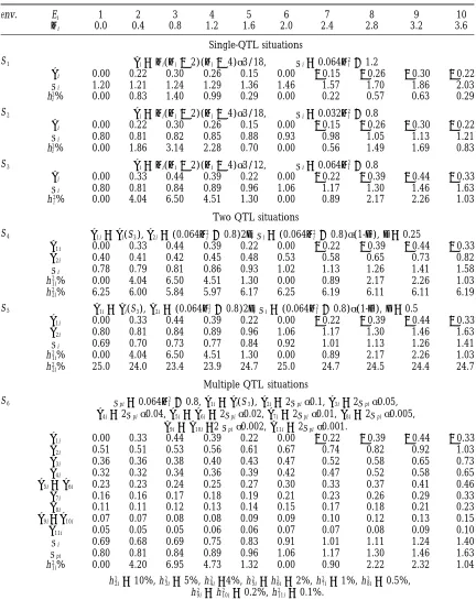
TABLE 1
Characteristics of the simulated multiple environment experiments with both the QTL substitution and residual standard deviation represented as functions of trait mean value
env. Ei 1 2 3 4 5 6 7 8 9 10
mi 0.0 0.4 0.8 1.2 1.6 2.0 2.4 2.8 3.2 3.6
Single-QTL situations
S1 ai5 mi(mi22)(mi24)√3/18, si50.064m2i 11.2
ai 0.00 0.22 0.30 0.26 0.15 0.00 20.15 20.26 20.30 20.22
si 1.20 1.21 1.24 1.29 1.36 1.46 1.57 1.70 1.86 2.03
h2
i% 0.00 0.83 1.40 0.99 0.29 0.00 0.22 0.57 0.63 0.29 S2 ai5 mi(mi22)(mi24)√3/18, si50.032m2i 10.8
ai 0.00 0.22 0.30 0.26 0.15 0.00 20.15 20.26 20.30 20.22
si 0.80 0.81 0.82 0.85 0.88 0.93 0.98 1.05 1.13 1.21
h2
i% 0.00 1.86 3.14 2.28 0.70 0.00 0.56 1.49 1.69 0.83 S3 ai5 mi(mi22)(mi24)√3/12, si50.064m2i 10.8
ai 0.00 0.33 0.44 0.39 0.22 0.00 20.22 20.39 20.44 20.33
si 0.80 0.81 0.84 0.89 0.96 1.06 1.17 1.30 1.46 1.63
h2
i% 0.00 4.04 6.50 4.51 1.30 0.00 0.89 2.17 2.26 1.03
Two QTL situations
S4 a1i5 ai(S3),a2i5(0.064m2i 10.8)2d,si5(0.064m2i 10.8)√(1-d2),d 50.25
a1i 0.00 0.33 0.44 0.39 0.22 0.00 20.22 20.39 20.44 20.33
a2i 0.40 0.41 0.42 0.45 0.48 0.53 0.58 0.65 0.73 0.82
si 0.78 0.79 0.81 0.86 0.93 1.02 1.13 1.26 1.41 1.58
h21i% 0.00 4.04 6.50 4.51 1.30 0.00 0.89 2.17 2.26 1.03
h22i% 6.25 6.00 5.84 5.97 6.17 6.25 6.19 6.11 6.11 6.19
S5 a1i5 ai(S3),a2i5(0.064m2i 10.8)2d,si5(0.064m2i 10.8)√(1-d2),d 50.5
a1i 0.00 0.33 0.44 0.39 0.22 0.00 20.22 20.39 20.44 20.33
a2i 0.80 0.81 0.84 0.89 0.96 1.06 1.17 1.30 1.46 1.63
si 0.69 0.70 0.73 0.77 0.84 0.92 1.01 1.13 1.26 1.41
h21i% 0.00 4.04 6.50 4.51 1.30 0.00 0.89 2.17 2.26 1.03
h22i% 25.0 24.0 23.4 23.9 24.7 25.0 24.7 24.5 24.4 24.7
Multiple QTL situations
S6 spi50.064m2i 10.8,a1i5 ai(S3),a2i52spi√0.1,a3i52spi√0.05,
a4i52spi√0.04,a5i5 a6i52spi√0.02,a7i52spi√0.01,a8i52spi√0.005,
a9i5 a10i52spi√0.002,a11i52spi√0.001.
a1i 0.00 0.33 0.44 0.39 0.22 0.00 20.22 20.39 20.44 20.33
a2i 0.51 0.51 0.53 0.56 0.61 0.67 0.74 0.82 0.92 1.03
a3i 0.36 0.36 0.38 0.40 0.43 0.47 0.52 0.58 0.65 0.73
a4i 0.32 0.32 0.34 0.36 0.39 0.42 0.47 0.52 0.58 0.65
a5i5 a6i 0.23 0.23 0.24 0.25 0.27 0.30 0.33 0.37 0.41 0.46
a7i 0.16 0.16 0.17 0.18 0.19 0.21 0.23 0.26 0.29 0.33
a8i 0.11 0.11 0.12 0.13 0.14 0.15 0.17 0.18 0.21 0.23
a9i5 a10i 0.07 0.07 0.08 0.08 0.09 0.09 0.10 0.12 0.13 0.15
a11i 0.05 0.05 0.05 0.06 0.06 0.07 0.07 0.08 0.09 0.10
si 0.69 0.68 0.69 0.75 0.83 0.91 1.01 1.11 1.24 1.40
spi 0.80 0.81 0.84 0.89 0.96 1.06 1.17 1.30 1.46 1.63
h21i% 0.00 4.20 6.95 4.73 1.32 0.00 0.90 2.22 2.32 1.04
h2
2i510%, h23i55%, h24i54%, h25i5h26i52%, h27i51%, h28i50.5%, h2
9i5h210i50.2%, h211i50.1%.
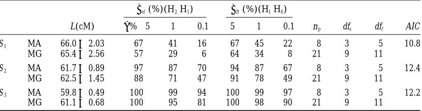
TABLE 2
Estimated location L(cM) and power of detection of QTL effect (bffor testing H1|H0) and
QTL3E interaction (befor testing H2|H1) employing the general (MG) and
approximated (MA) models in single-QTL situations
bet(%)(H2|H1) bft(%)(H1|H0)
L(cM) a%→5 1 0.1 5 1 0.1 np dfe dff AIC
S1 MA 66.062.03 67 41 16 67 45 22 8 3 5 10.8
MG 65.462.56 57 29 6 64 34 8 21 9 11
S2 MA 61.760.89 97 87 70 94 87 67 8 3 5 12.4
MG 62.561.45 88 71 47 91 78 49 21 9 11
S3 MA 59.860.49 100 99 94 100 99 97 8 3 5 12.2
MG 61.160.68 100 95 81 100 98 90 21 9 11
The results of 200 Monte-Carlo runs are presented for single-QTL situations (see Table 1). L is the estimated QTL location (the simulated value of L is 60 cM); a is significance level; np is the number of parameters specifying the model. To reduce np, the vector of mean valuesmiacross environments was calculated before starting the optimization procedure for the tests 3, 3a, and 3b (for either MA or MG); dffand dfeare the degrees of freedom for the tests of QTL presence (H1vs. H0) and QTL3E interaction (H2vs. H1), respectively.
detection of QTL3E interaction and the most precise ronments, which should be taken into account. One of
the possible ways to account for this correlation is through estimate of QTL location were obtained with model
MA3. It is not surprising that MA3is superior over MG. simultaneous analysis of multiple traits, taking the trait
values in different environments as different quantitative But less expected is the fact that the nonadequate
ap-proximations MA2and MA4were also superior over MG, traits (Korol et al. 1987, 1994, 1995; Jiang and Zeng
1995;Roninet al. 1995). However, the multiple trait
analy-whereas the poorest approximation MA1gave the closest
results to MG, but with fewer parameters. Thus, it is not sis limits the number of environments, because it is
asso-ciated with an increased number of parameters. The mandatory to have the adequate approximation to take
advantage of the proposed method. It will be sufficient approach proposed in this paper does not have this
drawback, but introduces other sources of distortions: to provide a good approximation. Nevertheless, how
can we decide about the adequate model, provided the (1) correlations caused by unaccounted QTLs, and (2)
approximated description of QTL dependence on envi-class of the approximation functions is chosen correctly?
To address the last question, the following procedure ronment based on the bioindication assumption.
Consider the first problem. We should now evaluate was employed. For each run, the data were analyzed
using all of the models (MA1–MA4, and MG), and mod- to what extent correlations between environments
caused by unaccounted QTLs may affect the efficiency
els that detected QTL 3 E interaction at the level of
significanceawere chosen. Then, the model that: (1) of the proposed approach. The second problem will be
treated in the next section and in thediscussion.
exceeded significantly (at some levela*) all of the more
simple models: (2) did not differ significantly (at a*) For the simulated cases of two QTLs segregating in
the mapping population (S4 and S5), we first analyzed
from more complex models was selected as adequate.
The general model also participated in this competition the consequences when the proposed approach of
ac-counting QTL3E interaction is applied, ignoring the
as the most complex one, because of the number of
parameters needed. The resulting distribution of the correlations caused by the effect of Q2/q2 (model 1,
Figure 3). Then, we re-evaluated the results by applying choices of the adequate model is presented in the last
three columns of Table 4. It allowed us to conclude the proper model (model 2, Figure 3). In these
simula-tions, we considered two situations of relative effects of
that: (1) model MA3 is an adequate model because it
was chosen in more than half of the runs where the the “target” QTL (Q1/q1) and of the cosegregating QTL
(Q2/q2): Q1/q1and Q2/q2have comparable effects on the
QTL3E interaction was detected, and with a frequency
that is threefold higher than the next best choice; (2) target trait though a1 , a2 (S4), and Q2/q2 is much
stronger than Q1/q1(S5). The residual variances2i of the
the models of the polynomial class were chosen 25–30
times more than the exact general model MG. More- trait within the QTL groups Q1/Q1 and q1/q1 was the
same in S3, S4, and S5.
over, even the simplest approximation, MA1, would be
selected 4– 6 times more frequently than MG. First, compare the accuracy of the QTL mapping
ob-tained employing model 1 for situation S4, with those
Two QTLs: When several QTLs segregate
simultane-ously in the mapping population, their effects will gener- of S3where only the effect of Q1/q1was simulated (the
situations S3 of Table 2 and S4, model 1, Figure 3). In
envi-both cases, the results clearly demonstrate the superior- Two possibilities exist for considering the effects of cosegregating QTLs in the mixture mapping model. ity of the approximated model MA. Hence, provided that
the effect of a cosegregating QTL, Q2/q2, does not consid- The first is to represent all QTL groups (four, in our
case, of two QTLs cosegregating in a doubled haploid
erably exceed the effect of the target QTL, Q1/q1, the
proposed approach provides accurate results even if or backcross population) in the likelihood function.
Although this procedure is not feasible for mapping
the effect of Q2/q2is ignored. However, this may not be
the case with larger effects of Q2/q2, as demonstrated multiple QTLs across the genome, it may be very useful
in cases of linked QTLs. The second is to include into
by the results for S5(model 1, Figure 3). In general, a
correct model should account for the genetic compo- the mixture model the effects of the cosegregating QTLs
as cofactors derived from regression analysis on marker nents of the residual variation in the alternative
geno-typic groups of the target QTL, causing correlation be- loci (Zeng1994;JansenandStam1994). The proposed
approximated method is equally applicable in both of
tween trait values across environments (e.g.,Jiangand
Zeng1995). This is also true for the method proposed these approaches. Here, we demonstrate it using the
first approach. Although this mixture formulation is here of mapping analysis with data measured in multiple
environments. more challenging technically, it allows for a proper
anal-ysis of potential variance effect of the cosegregating QTL (although we do not deal with this problem here). It is not obvious how to model the effect of a second QTL with regression cofactors. As was shown earlier, variance effect of a QTL may result in increased accuracy of the mapping model if it is included into the model, and may seriously reduce the accuracy with an
inade-quate model (Korolet al. 1996).
With two QTLs, four densitites fq1q1q 2q 2(x), fq1q1q2q 2(x),
fQ 1Q1q 2q2(x), and fQ 1Q 1Q 2Q2(x) should be considered. Conse-quently, in calculations of the maximum likelihood function, instead of four marker groups for a current interval, it is necessary to characterize 16 marker groups for any pair of nonadjacent intervals. The application results of the full MG model and the approximated polynomial MA model are presented in Figure 3 (model 2). It is noteworthy, that the proposed approximation of the environmental dependence of QTL effect as a function of the mean value of the trait in a given
environ-ment was applied not only to the target QTL Q1/q1, but
Figure 2.—Accuracy and precision of estimates of QTL also to the cosegregating Q
2/q2. This approach may be
effects across environments obtained by the general and ap- especially attractive when there are many cosegregating proximated single-QTL models applied to single-QTL data. QTLs with environmental dependent effects (e.g., as The graph represents estimated average trend and a sampled
regression cofactors on respective marker loci). This
95% vicinity of the p-dimensional point {ai/si, i51,... p} from
will result in far fewer parameters. As expected, the full
200 Monte-Carlo runs for situation S2(described in Table 1).
Open circles and light region are for the general model MG, model 2 increased the power of detection of Q1/q1effect black circles and shaded region are for the approximated on the trait x and (Q1/q1)3E interaction (not shown), model MA. The regions were obtained as follows. Let aiand as well as increased accuracy of estimates of the
chromo-sibe the QTL effect and the residual standard variation at the
some position of Q1/q1and of its effects by the
environ-ith environment (i...., p), and aijandsijbe the corresponding
ments (model 2, Figure 3). Again, MA had superior
estimates at j th run ( j51,..., 200). As a measure of discrepancy
of the estimated parameters from the expected, across envi- attributes than MG. This conclusion is also supported
ronments, we used the index by the values of AIC.
dj5√R(ai/si2aij/sij)2. Several QTL: As we could see before, a strong QTL, The sampled 95% volume is defined as a p-dimensional sphere, if not accounted by the model, may cause correlations
S0.95, of minimal radius with center at point {ai/si, i51,..., p}, between environments resulting in reduced accuracy which includes 95% of estimated results rj5(aij/sij, i51,..., p) of estimated parameters. Nevertheless, the distortion from the simulations. The sphere provides a 95% region of
caused by a QTL comparable with the target one (e.g.,
estimated curves aj(m(E )) in the plane of the estimated effects
exceeding the target effect no more than two times) is
{aij,m(Ei)}:
not dramatic (see Figure 3). Including the effects of
D0.955{aj(m(E )), aijP[min aij, max aij], i51,... p }.
cosegregating QTLs into the model solves this problem.
rjPS0.95 rjPS0.95
This can be done by combining the proposed approach
According to our calculations, the radius of S0.95is smaller for
pro-TABLE 3
Comparison of the general model with the polynomial approximations for the power of detection
of the QTL (bft), QTL3E interaction (bet), and the accuracy of QTL location (L)
bft(%)(H1|H0) bet(%)(H2|H1)
Model L(cM) a%→5 1 0.1 dff 5 1 0.1 dfe
MA1 60.660.74 98 90 74 3 96 85 63 1
MA2 61.060.59 99 98 92 4 98 95 84 2
MA3 59.860.49 100 99 97 5 100 99 94 3
MG 61.160.68 99 98 90 11 99 97 83 9
ME3 60.961.44 83 63 40 2
MA1, MA2, and MA3are the approximated models based on polynomials of first, second, and third degree, respectively, for the target QTL effect. Situation S3(see Table 1) is considered. The results are compared to the best single-environment model (ME3, for data from the environment 3 where the effect of the target QTL is the largest one).
portion of genetic variation for the analyzed trait may Table 5 (first row for N51,3,5). It is noteworthy, that in
this case employment of the asymptotic distribution for still remain in the residuals, because of combined effect
of many small QTLs. This residual genetic variation may the critical values of the test statistics gives seriously biased
upward estimatesbet5 bet(a) of the power of detection
be several-fold larger than the effect of the target QTL.
Would the resulting correlation between environments of Q1/q1 3 E interaction (compared to the estimates
bes 5 bes (a) obtained using Monte-Carlo simulations
preclude the application of the method?
To address this question, let us consider the case S6 with 5000 runs).
As we see from the foregoing results for the two QTL (for detailed specification see Table 1). Here, the genetic
variation of the trait depends on the target QTL (Q1/q1) situations (S4and S5in Figure 3), an unaccounted QTL
will not seriously affect the results for the target QTL if
(with an average h2z2.5% across environments) and 10
additional unlinked QTLs (Q2/q2–Q11/q11). The average its effect does not exceed the target one by too much
(e.g., not more than twofold). In the current situation
(across environments) effect of Q2/q2 was h2 z 10%,
whereas the combined average effect of Q3/q3–Q11/q11was S6, each of the simulated effects of Q3/q3–Q11/q11fit this
condition, whereas this is not true for their combined
15%. Thus, the total effect of Q2/q2–Q11/q11is 10-fold
com-pared to that of Q1/q1, whereas the effect of Q3/q3–Q11/q11 effect or for the individual effect of Q2/q2. It is interesting
to explore whether including Q2/q2 into the model as
is sixfold compared to that of Q1/q1. One may expect that
the power of detection of Q1/q13E interaction will be very a cofactor will improve the situation. This is indeed
an important question, because in practice sufficiently
low if the segregation of Q2/q2–Q11/q11 is not accounted
for by the model, hence causing correlation between the strong QTLs can be compensated in such a way (Jansen
andStam1994;Zeng1994), but this does not guarantee
environments. This is indeed the case as can be seen from
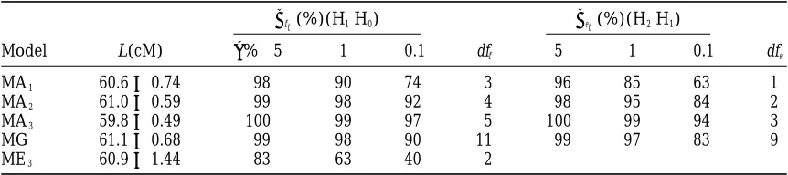
TABLE 4
Comparison of the general model with the polynomial approximations for the detection
power of QTL3E interaction (be), and accuracy of QTL location (L)
be(%) fM
Model L(cM) a%→5 1 0.1 df a%→5 1 0.1
MA1 62.061.46 88 (88) 68 (69) 48 (46) 1 0.18 0.16 0.13
MA2 61.161.31 92 (92) 78 (77) 56 (59) 2 0.18 0.17 0.15
MA3 61.760.89 96 (97) 86 (87) 66 (70) 3 0.54 0.49 0.45
MA4 61.660.92 95 (95) 80 (82) 61 (61) 4 0.05 0.05 0.05
MG 62.561.45 88 71 47 9 0.03 0.03 0.03
Total frequency of cases where QTL3E interaction was detected 0.98 0.90 0.78
Figure 3.—Accuracy of estimates of QTL effects across environments obtained by the general and approximated models
applied to two-QTL data. Here model 1 and model 2 denote a single- and two-QTL mapping models. In situation S4, the effects of simulated unlinked QTLs were: average h2%≈2.5 (range 0–6.5) for QTL1and 6.0 (range 5.84–6.25) for QTL2, respectively; in situation S5, the simulated effects were: average h2% ≈2.5 (range 0–6.5) for QTL1and 24.0 (range 23.4–25.0) for QTL2, respectively. A IC is the Akaike’s information criterion which takes into account the cost of increased number of parameters in the model (Bozdogan1987).
that the residual variation caused by many small polygenes andbes) in spite of the noise caused by Q3/q3–Q11/q11. It
would be quite desirable to get some idea of the dis-will not exceed the target effect several times over, thus
preventing the application of the proposed method. torting effect of the correlations caused by joint action
of the unaccounted QTLs Q3/q3–Q11/q11. Therefore, for
The data presented in the second row of Table 5
show that including Q2/q2as a cofactor into the model comparison we provide in the third row the results for
the case where all the residual genetic variation caused substantially improved the situation by increasing the
detection power of Q1/q13 E interaction from two- to by Q3/q3–Q11/q11 is replaced by nongenetic variation.
We can conclude that distortion of the basic model
fivefold (for a, ranging from 0.05 to 0.001) and the
precision of Q1/q1estimated location more than twofold. assumption of “no correlation between environments”
caused by the presence of Q3/q3–Q11/q11, which
collec-Note that in this case the x2 distribution appeared to
be a very good approximation for the distribution of tively exceed by a factor of six the effect of the target
QTL Q1/q1, is incomparably smaller than that caused by
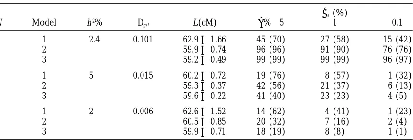
TABLE 5
The effect of cofactors on the power of detection of QTL3E interaction (be),
and accuracy of QTL location (L)
be(%)
N Model h2% D
gei L(cM) a%→5 1 0.1
1 1 2.4 0.101 62.961.66 45 (70) 27 (58) 15 (42)
2 59.960.74 96 (96) 91 (90) 76 (76)
3 59.260.49 99 (99) 99 (99) 96 (97)
3 1 5 0.015 60.260.72 19 (76) 8 (57) 1 (32)
2 59.360.37 42 (56) 21 (37) 6 (13)
3 59.660.22 41 (40) 23 (23) 4 (5)
5 1 2 0.006 62.661.52 14 (62) 4 (41) 1 (23)
2 60.560.85 20 (32) 7 (16) 2 (4)
3 59.960.71 18 (19) 8 (8) 1 (1)
The power of the test was obtained using Monte-Carlo simulations (see text); (corresponding results based onx2asymptotic distribution of the test statistic are given in brackets). Data of the situation S6(see Table 1) were used with the target QTL on chromosome N (N51, 3 or 5). Three models of the analysis of the residual variation were employed: (1) the cofactors are totally ignored; (2) the effect of the strongest QTL is fitted using two-QTL mixture model; (3) the genetic component of the residual variation is replaced by the equivalent nongenetic variation. Dgeiis the variance of QTL 3 E interaction for the target QTL; h2% is the averaged heritability over environments attributed to the target QTL.
a single QTL, Q2/q2, which exceeds the target QTL only 1996). Thus, according to the simulation results of the
previous section, even if one ignores the effects of other by a factor of four. The same analysis was conducted
when instead of Q1/q1 another QTL was considered as genomic segments when dealing with markers of
chro-mosome 1, we did not expect serious reduction in the
a target one (Q3/q3or Q5/q5). The results are presented
in the remainder of Table 5 and manifest the same efficiency of the mapping analysis. As shown in Figure 1,
the estimates of ai for this trait obtained for separate
pattern.
Missing data: One can hardly expect that all geno- environments can be approximated as a quadratic para-bola of the mean value of the trait over the environments. types will be perfectly represented in all of the
environ-ments where the experiment was conducted. Some data This approximation was used to construct a combined
model for testing QTL3E interaction effect and to
esti-will be missed, hence it is of interest to get some idea
how it could affect the power of QTL 3 E detection. mate the QTL location on chromosome 2 (Table 7).
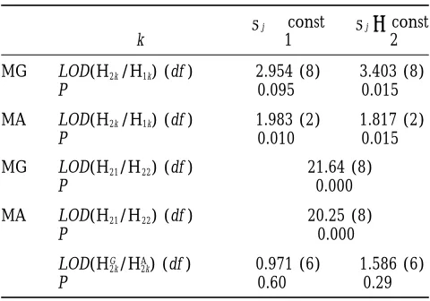
The first step was to decide whether variation ins2
i
Our approximate model allows us to treat this problem
easily. It appeared that with a large number of environ- is significant and should be included into the model.
Our prior trial showed that polynomial regression of ments, even if a large proportion of genotypes is not
represented in each environment, the resulting power s2
i on mean trait value is nonsignificant (data not
shown). Thus, the hypotheses “constants2
i 5 s2across
of the test of QTL3E interaction and location accuracy
of the target QTL are quite high. Monte-Carlo simula- environments” and “variable s2
i across environments”
were contrasted employing two models to describe the tions presented in Table 6 illustrate this point. It is
noteworthy, that if only 20–50% of the data are available dependence of aion environment: the general model
MG and quadratic approximation MA. Both approaches in each of the 50–100 environments, the approximated
model is still very satisfactory even when a suboptimal reject the hypothesis of constants2
iat a highly significant
level (with LOD values 21.64 and 20.25 for MG and MA,
approximation was used (compare the results for MA1,
MA2, and MA3for the two examples with the situation respectively). Therefore, we should test for the presence
of QTL 3 E interaction given environmental-specific
S4). Clearly, an attempt to apply the general model
would mean an unrealistic task of estimation of about s2
i. Here, we can see the advantage of the proposed
approach. Indeed, with the polynomial approximation 100–200 parameters, in contrast to our model which
needs only eight parameters. of ai for H2 {ai ? const}, the hypothesis H1 {ai 5 a 5
const} is rejected at the significance level of P50.010,
Example of application:The trait “alpha amylase
activ-ity” from a barley QTL3E study presented in Figure 1 while based on the general model MG we can get only
P5 0.095.
(see Hayeset al. 1993, 1996) was used to demonstrate
the utility of the proposed procedure. From previous An important question is whether the two models,
MA or MG, differ significantly provided H2{ai?const}
analyses, the largest QTL effect for this trait was
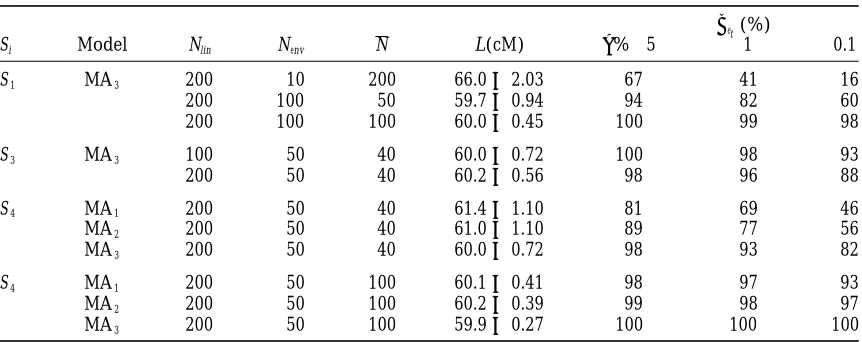
con-TABLE 6
The effect of missing data on the power of detection of QTL3E interaction and accuracy of QTL
location when the number of environments is large
bet(%)
Si Model Nlin Nenv N L(cM) a%→5 1 0.1
S1 MA3 200 10 200 66.062.03 67 41 16
200 100 50 59.760.94 94 82 60
200 100 100 60.060.45 100 99 98
S3 MA3 100 50 40 60.060.72 100 98 93
200 50 40 60.260.56 98 96 88
S4 MA1 200 50 40 61.461.10 81 69 46
MA2 200 50 40 61.061.10 89 77 56
MA3 200 50 40 60.060.72 98 93 82
S4 MA1 200 50 100 60.160.41 98 97 93
MA2 200 50 100 60.260.39 99 98 97
MA3 200 50 100 59.960.27 100 100 100
Nlinis the total number of genotypes (lines) in the mapping population, Nenvis the number of environments, and N is the mean number of genotypes scored per environments. To generate the data, the initial form of the dependence of the QTL on environment was used as presented in Table 1, but with a correspondingly smaller step in changes of the independent variable.
sidered situations, i.e., withs2
i 5 const ands2i ?const, large (in fact, unlimited) number of “anonymous”
envi-using LOD scores (see the last section of Table 7). In ronments. Expressing the dependence of a QTL effect
no case was the difference significant, so that MA pro- on environmental conditions as a function of
environ-vides the same solution as MG, but the approximated mental mean value of the trait can also be applied to
model is preferable because of a lower number of multiple QTLs from independent genomic regions.
needed parameters. In other words, MA extracts from Therefore, the proposed approach could be very helpful
the data the same information on variation of the QTL in coping, albeit in an approximate form, with a difficult
effect ai across environments as MG, but does it more problem of QTL mapping analysis, i.e., rapid increase
efficiently. in the number of parameters with increasing number
of effective QTLs and environments. This improves our ability to efficiently extract more mapping information
DISCUSSION when more environments are used to evaluate the
quan-titative trait. The conducted simulations and the example of barley
In addition to the large number of parameters to be multiple environments experiment demonstrate the
estimated, the general model MG of QTL 3E
interac-utility of the proposed approximate approach for
analyz-tion fails to account for correlaanalyz-tion between
environ-ing QTL3E interaction. Its main benefit is the ability to
ments caused by cosegregating QTLs not included into use data collected from a large number of environments
the model. While the first problem is not critical for without the necessity of increasing the number of
pa-our method, the second one may be more serious. The rameters. Earlier, an elegant solution to this problem
foregoing simulations showed that unaccounted QTLs
was proposed byJansenet al. 1995. Their QTL mapping
with a strong individual effect may indeed reduce the model includes in an obvious way the terms describing
power of detection of QTL 3 E interaction and the
the effects of the target QTL and regression cofactors
accuracy of parameter estimation by the proposed ap-of cosegregation QTL, the effects ap-of multiple
environ-proximated method. Therefore, including such QTLs as
ments, and the terms of QTL3E interactions. However,
cofactors into the model is mandatory for applications. such an analysis is limited by situations where the
envi-However, such a compensation cannot be perfect and ronments can be obviously characterized by some
physi-a significphysi-ant genetic component mphysi-ay remphysi-ain in the re-cal attributes. When such characteristics are not
avail-sidual variation. An important question is whether this
able, the application of the general QTL3E mapping
residual genetic variation, which can be several-fold model (our foregoing MG model) is accompanied by
larger than the effect of the target QTL, will produce a tremendous number of parameters involved in the
correlation between the environments precluding the model. The method proposed in this paper overcomes,
application of the method. Our simulations allowed us though in an approximate form, both these obstacles,
assump-TABLE 7 not valid. If the opposite is true, i.e., if the dependence of the QTL effect on environmental conditions can
Detection of QTL3E interaction in a barley
indeed be presented in the form of regression on mean dihaploid population scored over nine environments (for
values or any other bioindicators, then the proposed a QTL of chromosome 1 affecting ‘alpha amylase
activity’; see Hayes et al. 1996) approximated method proved to give a higher detecting
power of QTL3E interaction compared to the precise
sj?const sj5const general model (MG). Thus, one can start the procedure
k 1 2 using the approximated method, though the general
model can also be applied in parallel if the number of
MG LOD(H2k/H1k) (df ) 2.954 (8) 3.403 (8)
environments is not too large, so that the number of
P 0.095 0.015
parameters for MG is not unrealistically large. However,
MA LOD(H2k/H1k) (df ) 1.983 (2) 1.817 (2)
if the approximated analysis revealed no significant
P 0.010 0.015
QTL3E interaction, does it really mean an
indepen-MG LOD(H21/H22) (df ) 21.64 (8) dence of the QTL effect from environmental
condi-P 0.000
tions? Or, alternatively, the interaction may exist, but it
MA LOD(H21/H22) (df ) 20.25 (8) cannot be represented as a regression of the target QTL
P 0.000 effect on the mean values of the trait or some other
bioindicators?
LOD(HG2k/HA2k) (df ) 0.971 (6) 1.586 (6)
Consider one of the possible ways to cope with this
P 0.60 0.29
problem. If the general model is applicable, i.e., the
We used the index k to denote two types of models
corre-number of parameters is not too large, it may be used
sponding to equal (k 5 1) vs. nonequal (k 5 2) residual
as a tool to answer the foregoing question. Rejection of
variances across environments. Therefore, H11and H12
hypoth-the H0 hypothesis “no QTL 3 E interaction” by MG
eses here assume the presence of a QTL effect with constant
and varying residual variances, respectively. Correspondingly, will mean that our basic assumption (regression on the
H21and H22assume the presence of a QTL with varying effect bioindicator) does not fit the data. If the number of and constant and varying residual variances, respectively. To test
environments is too large, the general model can be
whether the two models, MA or MG, differ significantly, provided
applied for randomly chosen groups of environments.
H2{aj?const} is true, both situations, i.e., withs2t 5const and
Then, the significance of the interaction may be evalu-s2
i ?const, were considered using LOD score, LOD(HG2k/HA2k)
(see the last section of the table). ated from the obtained distribution of the tests using
the Bonferroni correction. For example, with N5100
environments, one can produce k 5 20 samples, each
tion of “no correlation between environments” caused including data of m 5 10 randomly chosen
environ-by the segregation of several small QTLs, which collec- ments. Let a be the accepted level of significance for
tively exceed by a factor of six the effect of the target the QTL 3 E interaction test for the whole set of the
QTL, is much smaller than that caused by a strong single samples. Then, assuming independence of these
sam-QTL, which exceeds the target QTL by only a factor of ples, one can reject the H0hypothesis if at least one of
four (see Table 5). Thus, undetectable small QTLs will the samples achieved the significance level of a/k.
not attenuate seriously the resolution power of the pro- Clearly, due to the postulated independence, which is
posed method, even if their combined effect is several- not the case for mk . N, this is a conservative test of
fold higher than that of the target QTL. QTL3E interaction. Nevertheless, it seems preferable
An important question is how to reveal the adequate to us than the standard way of multiple-environment
approximation of the QTL3E interaction. With simu- data analysis when the data from each environment are
lated data, it is easy to compare the adequate and the treated separately, and the final conclusion is derived
nonadequate approximations simply because we know from the analysis of the estimated QTL effects across
the degrees of the polynomials employed in the simula- environments (Patersonet al. 1991;Stuberet al. 1992;
tions. However, the situation will be quite different when UtzandMelchinger 1996).
real data will be analyzed. Thus, the decision about The foregoing test based on the general model may
the adequacy of the approximation should be justified result in the same conclusion as the approximated model,
statistically, i.e., we should decide about the adequate i.e., “no QTL3E interaction.” By contrast, if the general
model, provided the class of the approximation func- model allowed us to detect QTL 3 E interaction, but
tions is chosen correctly. This allows us to conclude the approximated model did not, it will indicate that the
that: (1) the adequate model MA3was the best, i.e., it proposed bioindicator(s) is not informative and other
ex-was chosen in more than half of the runs where the planatory factors could be found. Further studies are
QTL3E interaction was detected and with a frequency needed to develop more optimal algorithms of application
that was threefold higher than the next best choice. of the proposed approach when applied to a large number
The last and most difficult problem is how to recog- of environments (and when direct utilization of the
Korol, A. B., A. A. ZhuchenkoandA. P. Samovol,1981 Linkage
form, the drawbacks of the proposed method are
compen-between loci of quantitative characters and marker loci. III. The
sated by the possibility of working with an unlimited num- bias of estimates upon disturbance of basic assumptions. Genetica
(in Russian) 17: 1234–1247.
ber of environments with missing data, and at a
remark-Korol, A. B., I. A. PreygelandN. Bocharnikova, 1987 Linkage
able reduction in the number of parameters needed, as
between loci of quantitative traits and marker loci. 5.
Simultane-compared to the usual way of testing for QTL3E interac- ous analysis of a set of marker and quantitative triats. Genetika
(USSR) 23: 1421–1431.
tions based on ANOVA treatment of QTL estimates
ob-Korol, A. B., I. A. PreygelandS. I. Preygel,1994 Recombination
tained on the basis of single-environment analysis.
Variability and Evolution. Chapman & Hall, London.
Korol, A. B., Y. I. RoninandV. M. Kirzhner,1995 Interval mapping We are grateful to the North American Barley Genome Mapping
of quantitative trait loci employing correlated trait complexes. Project (Dr.P. M. Hayes) for the data set employed in our illustrative
Genetics 140: 1137–1147. example. We are very thankful to the anonymous referees for their
Korol, A. B., Y. I. Ronin, Y. Tadmor, A. Bar-Zur, V. M. Kirzhner relevant comments and suggestions that assisted in improvement of
et al., 1996 Estimating variance effect of QTL: an important the manuscript. This work was supported by the Israeli Ministry of prospect to increase the resolution power of interval mapping. Absorption and Ministry of Science and the Ancell-Teicher Research Genet. Res. 67: 187–194.
Foundation for Genetics and Molecular Evolution. Lander, E. S.,andD. Botstein,1989 Mapping Mendelian factors underlying quantitative traits using RFLP linkage maps. Genetics
121:185–99.
Paterson, A. H., S. Damon, J. D. Hewitt, D. Zamir, H. D. Rabinow-itchet al., 1991 Mendelian factors underlying quantitative traits LITERATURE CITED
in tomato: comparison across species, generations and environ-ments. Genetics 127: 181–197.
Asins, M. J., P. Mestre, J. E. Garcia, F. DicentaandE. A. Carbonell,
Rendel, J. M.,1967 Canalization and Gene Control. Academic Press, 1994 Genotype3environment interaction in QTL analysis of
London. an intervarietal almond cross by means of genetic markers. Theor.
Romagosa, I., S. E. Ullrich, F. HanandP. M. Hayes,1996 Use Appl. Genet. 89: 358–364.
of additive main effects and multiplicative interaction model in Baker, R. J.,1996 Recent research on genotype-environmental
inter-QTL mapping for adaptation in barley. Theor. Appl. Genet. 93: action. Proceedings of the 5th International Oat Conference
30–37. and 7th International Barley Genetics Symposium, Saskatoon,
Ronin, Y. I., V. M. KirzhnerandA. B. Korol,1995 Linkage between Saskatchewan, Canada, pp. 235–246.
loci of quantitative traits and marker loci. Multi-trait analysis with Beavis, W. D.,andP. Keim,1996 Identification of QTL that are
a single marker. Theor. Appl. Genet. 90: 776–786. affected by environment, in Genotype by Environment Interactions,
Sari-Gorla, M., T. Calinski, Z. KaczmarekandP. Krajewski,1997 edited byM. S. KangandH. Gauch, Jr.CRC Press, Inc.
Detection of QTL-environment interaction in maize by a least Bozdogan, H.,1987 Model selection and Adaike’s information
cri-squares interval mapping method. Heredity 78: 146–157. terion (AIC): the general theory and its analytical extention.
Stuber, C. W., S. E. Linkoln, S. E. Wolff, T. HelentjarisandE. S. Psychometrika 52: 345–370.
Lander,1992 Identification of genetic factors contributing to Eberhard, S. A.,andW. A. Russel,1966 Stability parameters for
heterosis in a hybrid from two elite maize inbred lines using comparing varieties. Crop Sci. 6: 36–40.
molecular markers. Genetics 132: 823–839. Falconer, D. S.,1981 Introduction to Quantitative Genetics. Longman
Tinker, N. A.,andD. E. Mather,1995 Methods for QTL analysis Scientific & Technical, Essex, UK.
with progeny replicated in multiple environments. J. Quant. Trait Gilbert, N.,1961 Polygene analysis. Genet. Res. 2: 96–102.
Loci 1 (2). http: //probe. nalusda.gov: 8000/otherdocs/jqtl/jqtl Hayes, P. M.,1994 Genetic stocks available through the North
Amer-1995-02/jqtl16r2.html ican Barley Genome Mapping Project. Barley Genet. Newsl. 24:
Tiret, L., L. AbelandR. Rakotovao,1993 Effect of ignoring geno-113–116.
type-environment interaction on segregation analysis of quantita-Hayes, P. M., B. H. Liu, S. J. Knapp, F. Chen, B. Joneset al., 1993
tive traits. Genetic Epidemiology 10: 581–586. Quantitative trait locus effects and environmental interaction in
Utz, H. F.,andA. E. Melchinger,1996 PLABQTL: a program for a sample of North American barley germplasm. Theor. Appl. composite interval mapping of QTL. J. Quant. Trait Loci 2 (1). Genet. 87: 392–401.
http: / / probe.nalusda.gov:8000 / otherdocs/jqtl/jqtl1996-01 / Hayes, P. M., G. BricenoandD. Matthews,1996 The Steptoe3
utz.html Morex barley mapping population. http://probe.nalusda.gov:
Via, S., andR. Lande,1987 Evolution of genetic variability in a 8300/edi-bin/browse/graingenes spatially heterogeneous environment: effects of genotype-envi-Himmelblau, D. M.,1972 Applied Nonlinear Programming.
McGraw-ronment interaction. Genet. Res. 49: 147–156.
Hill, New York. Weller, J. I.,1986 Maximum likelihood techniques for the mapping Jansen, R. C.,andP. Stam,1994 High resolution of quantitative
and analysis of quantitative trait loci with the aid of genetic mark-traits into multiple loci via interval mapping. Genetics 136: 1447– ers. Biometrics 42: 627–640.
1455. Wilks, S. S.,1962 Mathematical Statistics. John Wiley & Sons, New Jansen, R. C., J. M. Van Ooijen, P. Stam, C. ListerandC. Dean,
York.
1995 Genotype-by-environment interaction in genetic mapping Wu, R.,andR. F. Stettler,1997 Quantitative genetics of growth of multiple quantitative trait loci. Theor. Appl. Genet. 91: 33–37. and development in Populus. II. The partitioning of genotype3 Jiang, C.,andZ.-B. Zeng,1995 Multiple trait analysis and genetic
environment interaction in stem growth. Heredity 78: 124–134. mapping for quantitative trait loci. Genetics 140: 1111–1127. Zeng, Z.-B.,1994 Precision mapping of quantitative trait loci. Genet-Knott, S. A.,andC. S. Haley,1992 Aspects of maximum likelihood ics 136: 1457–1468.
methods for mapping of quantitative trait loci in line crosses.