Volume 2010, Article ID 461538,28pages doi:10.1155/2010/461538
Research Article
Tracking Algorithms for Multistatic Sonar Systems
Martina Daun
1and Frank Ehlers
21Department of Sensor Data and Information Fusion (SDF), Fraunhofer FKIE, Neuenahrer Straße 20, 53343 Wachtberg, Germany 2NATO Undersea Research Centre (NURC), 19126 La Spezia, Italy
Correspondence should be addressed to Frank Ehlers,[email protected]
Received 3 December 2009; Revised 5 May 2010; Accepted 23 June 2010
Academic Editor: Christoph F. Mecklenbr¨auker
Copyright © 2010 M. Daun and F. Ehlers. This is an open access article distributed under the Creative Commons Attribution License, which permits unrestricted use, distribution, and reproduction in any medium, provided the original work is properly cited.
Activated reconnaissance systems based on target illumination are of high importance for surveillance tasks where targets are nonemitting. Multistatic configurations, where multiple illuminators and multiple receivers are located separately, are of particular interest. The fusion of measurements is a prerequisite for extracting and maintaining target tracks. The inherent ambiguity of the data makes the use of adequate algorithms, such as multiple hypothesis tracking, inevitable. For their design, the understanding of the residual clutter, the sensor resolution and the characteristic impact of the propagation medium is important. This leads to precise sensor models, which are able to determine the performance of the surveillance team. Incorporating these models in multihypothesis tracking leads to a situationally aware data fusion and tracking algorithm. Various implementations of this algorithm are evaluated with the help of simulated and measured data sets. Incorporating model knowledge leads to increased performance, but only if the model is in line with the physical reality: we need to find a compromise between refined and robust tracking models. Furthermore, to implement the model, which is inherently nonlinear for multistatic sonar, approximations have to be made. When engineering the multistatic tracking system, sensitivity studies help to tune model assumptions and approximations.
1. Introduction
Submarines operate covertly, hidden under the surface of the sea. Maneuvering silently is their greatest threat. To detect a submarine, active sound is transmitted, which is then reflected by the submarine and recorded by a sensor. This is called active sonar. In active sonar, different types of signals are used: in particular, in this paper, we study frequency-modulated sweeps (FM), which provide a good-range resolution, and continuous wave signals (CW), which provide Doppler information. However, submarine designers build submarine hulls in shapes that give them stealth even for active sonar: in cases when just a single source and a single receiver are used, the submarine can minimize by clever navigation the presented target strength to disappear in the background. The background consists of noise and, which is even worse from a tracking point of view, of aspect-dependent reverberation. As a result, false alarms with geometry-dependent statistics occur. Consequently, an antistealth setup consists of multiple sources and receivers.
This makes it almost impossible for the submarine to hide its strong echo returns. This concept is called multistatic active sonar. Covert receivers exploit the operational benefit that the submarine cannot determine whether it is detected or not. Exploiting the full multistatic setup will therefore result in additional detection probabilities.
The aim of target tracking is to determine the condi-tional probability of the target state given the measurement history of all data generated by the available multistatic source receiver pairs and, therein, from the available “signal channels” (FM or CW). A theoretically optimal approach for this tracking and fusion exists in the Bayesian framework [1]. For practical considerations, and to result in a real-time-capable algorithm, we applied specific techniques (adopted from ground moving target indication [2]) and evaluated their performance with the help of data sets from real measurements at sea and with simulated data sets.
(S/R) pairs, a correct association between the receivers’ data and all sound-reflecting objects is necessary. In the noisy and reverberant ocean environment, finding the true data associations is impeded by false alarms and missed detections. Even harder, the ocean only provides a fading channel for sound transmissions. Furthermore, the accuracy of measured contact and environmental data is limited by the given variability of the underwater sound channel and by budget or feasibility constraints on the quality and number of measurements.
Sonar performance modelling is able to describe the stochastic effects in the multistatic measurement. Together with a precise modelling of geometrical and kinematical features [3], a sensor model is constructed that becomes part of a sequential tracking algorithm, in this paper, it is the multihypothesis tracking (MHT) algorithm. Only the correct modelling allows a successful multisensor data fusion and by this the full exploitation of the multistatic sonar setup.
The MHT algorithm has a Kalman filter kernel. Because the sensor model is nonlinear, approximations are necessary and can be implemented in four different ways: linear transformation of each measurement in Cartesian coordi-nates with tracking in the Cartesian system (Cartesian L), unscented transformation (UT) [4] of each measurement in Cartesian coordinates with tracking in the Cartesian system (Cartesian UT), extended Kalman filtering (EKF) [5], and unscented Kalman filtering (UKF) [4].
The novel contribution of the paper is a precise and “situ-ationally aware” fusion strategy for multistatic measurements inside the MHT framework.
Key prerequisites to achieve this are
(i) a precise modelling of the deterministic features in a multistatic measurement and incorporation of this measurement modelling in the framework of the Unscented Kalman Filter (Section 3) and
(ii) an optimal data fusion which can be found by weight-ing the fusion input by its quality. Quality is evaluated by solving the sonar equation for each source-receiver geometry, each ping, and each hypothetic target. The performance of the adaptive scheme is compared to static fusion schemes. Details are provided in
Section 7.
Furthermore, we are applying
(i) for bistatic measurements an extension to the lin-earization methods in [6] a strategy to incorpo-rate probabilistic features based on the Unscented Transformation. Additionally strategies based on the idea of UKF and EKF are developed in Section 6. The performance of the resulting four tracking architectures (Cartesian L, Cartesian UT, EKF, and UKF) is evaluated with the help of Monte Carlo simulations inSection 8.2
(ii) an algorithm for ground moving target indication to fuse contacts with additional Doppler information (Section 7.4).
The remainder of this paper is organized as follows. In
Section 2, we describe the multistatic sonar system. In
Sections3 and4, we model deterministic and probabilistic features of the multistatic sonar measurements. We specify the structure of a sequential tracking algorithm inSection 5, in particular the multihypothesis tracking algorithm (MHT), and adapt it for its application to multistatic sonar data in
Section 6. InSection 7, we address the problem of finding an adequate fusion architecture. Results with experimental and simulated data are provided inSection 8. We summarize our findings inSection 9.
2. Multistatic Sonar
Multistatic active sonar involves multiple entities transmit-ting signals and receiving echoes. Receivers can be kept covert if they are spatially separated from the transmitter. Of interest for this paper is a system setup that consists of fixed arrays (Figure 1). This is used to create a barrier against submarine entry. The major advantage of multistatic sonar system is that there are more “ears” in the water to improve the detection, localization and identification of undersea objects, which results in a reduced false alarm rate.
Today’s submarines are designed to be stealthy. By clever navigation, they can avoid detection from a monostatic active sonar. But a multistatic system has additional detection opportunities in comparison to a monostatic system. To exploit this benefit, the data gathered at different transmitter-receiver pairs must be associated. In other words, data fusion has to find the best combination out of all possible detections from all source-receiver pairs in a series of measurements. Sonar performance prediction modelling shows that only rarely two distributed sensors have a similar quality on a specific ping of the target track. Therefore, data fusion algorithms must be based on realistic modelling of sensor performance for each sensor, each ping, and each target. Data are weighted so that data, which are considered more accurate or valid, are given more weight in the algorithms. This is implementing a “situationally aware” tracking, which has an improved performance compared to architectures of tracking algorithms with fixed sensor performance setting.
In practice, the software system for multistatic active sonar involves three steps.
(1) The collation of contact files from the networked receiving buoys: there is a contact file for each ping (i.e., transmission of an acoustic signal and each receiver). Each contact file contains for each detected echo the measurement vector (depending on the associated CW/FM channel)
zCW=ϕ,τ, ˙rT, zFM=ϕ,τT, (1)
whereτ is the time of arrival, which is the bistatic rangerdivided by the speed of sound, ˙ris the bistatic range-rate, which is proportional to the Doppler, and
ϕis the azimuth measurement. For each contact the associated SNR-value is also stored.
Radio antenna
Radio mast
Radio buoy
Surface electronics Batteries
Cable
Ballast Acoustic
aperture
Submerged electronics
Ballast
Radio antenna
Radio buoy Surface electronics Batteries
Cable Acoustic aperture
Submerged electronics
Ballast
(a) DEMUS system
(b) Stationary receiver (c) Stationary acoustic source
Figure1: Illustration of a stationary multistatic sonar system (a). A prototype of a stationary receiving system is shown in (b). As an acoustic source, the stationary system shown in (c) has been used. The system with three receivers and the source is called DEMUS. See [7,8] for further information.
is a priori known and that there is evidence that this will improve the localization accuracy.
(2) The use of data fusion and tracking algorithms to combine the information in the contact files. This is the topic of this paper.
(3) The output of the algorithm into a human computer interface that can facilitate interpretation of the data. The output consists of a set of tracks that is updated in real-time as a new contact file is received. Each track must include the position, speed, and course of the target. This information is stored in the state vectorx.
3. Modelling Deterministic Features of
Multistatic Sonar
Letq =(x,y)T be the target position ands=(sx,sy)T and
o = (ox,oy)T the position of the source, and the receiver,
respectively. The receiver orientation (heading) is given byϑ, c.f.Figure 2. Then, the measurements can be expressed as
ϕ=arctan
x−ox y−oy
−ϑ,
τ=q−sc+q−o S
,
˙
r= ∂τ∂tcS,
(2)
where | · · · | denotes the Euclidian norm and cS is the propagation speed of sound in water.
3.1. Timing. Assuming the target velocity to be constant between two consecutive pings, the standard bistatic range measurement equation (2) (wherer=τ·cS) is replaced by
r=q+t0q˙−s+q+t0q˙−o, (3)
q=(x,y)T
s=(sx,sy)T
o=(ox,oy)T
q−s o−q
North
East −ϕ ϑ
Figure2: Bistatic setup; sound from source atsis reflected by the target atqand received ato.ϑis the heading of the receiver relative to North.
then we need to solve
(x+t0x˙−sx)2+ (y−t0y˙−sy)2 = t0cS. Calculations yield
t0=
q−sTq˙
c2
S−vT2
+
q−sTq˙2
c2
S−v2T
2 +
q−s2
c2
S−v2T
, (4)
withvT= |q˙|.
3.2. Range-Doppler Ambiguity. Relative movement between source, target, and receiver leads to frequency shiftsΔf in the received target echo. For FM signals, the matched filter converts these frequency shifts into shifts of detection time. Assuming perfect knowledge of the relative movement, these shifts can be corrected. The frequency characteristics fmin+ t(fmax − fmin)/ΔS = fmin+Δf delivers the time shiftt =
ΔfΔS/(fmax− fmin), whereΔSis the duration of the signal. The modified measurement equation for range is therefore given by
r=q−s+q−r+r˙ 2
fmax+ fmin
fmax−fmin ΔS, (5)
where the bistatic range-rate ˙ris given by
˙
r =
q−sTq˙−s˙
q−s +
q−oTq˙−o˙
q−o . (6)
Thus, the measurement equation is corrected by the esti-mated Doppler value (calculated from the estiesti-mated target position and velocity).
Remarks. The speed of sound waves is slow compared to electromagnetic waves. Therefore, a precise modelling of geometric features and Doppler effects is important. Without this precise modelling geometry-dependent errors estimat-ing, the target state hampers the correct contact association and finally the optimal exploitation of the multistatic data fusion.
Of course, correction for both features (timing and range-Doppler ambiguity) can be done simultaneously. The combined range equation is
r=q+t0q˙−s+q+t0q˙−o+ ˙
r
2
fmax+fmin
fmax−fmin ΔS, (7)
For further reference in this paper, an algorithm implement-ing equation (4) is called “TiCor”, (5) is “DoCor”, and (6)
Table1: Probabilistic features in the underwater sound channel.
Probabilistic features in the underwater sound channel are (1) floating, drifting, or rotating sensor platforms;
(2) rapidly changing (spatially and temporally) environmental conditions;
(3) multipath arrivals with very variable structure;
(4) high noise levels at sensors; (e.g., on towed array due to flow noise or on stationary systems due to passing vessels); (5) strong fading;
(6) for active sonar a highly cluttered and aspect-dependent reverberation background.
is “DoTiCor”. Note that in (4), (5), and (6), the range is a function of the target velocity.
4. Modelling Probabilistic Features of
Multistatic Sonar
Probabilistic features in the underwater sound channel must be reflected in the tracking algorithm. Table 1 lists the probabilistic features influencing the sonar measurement.
4.1. Mapping of Uncertainties in the Measurements to Carte-sian Coordinates. The effect of items (1) to (2) inTable 1is that only estimates for sound speedcS, receivero,and source
s positions as well as receiver orientation (heading) ϑ are available.
Hence, we model the uncertainty following [9] byo ∼ N(o;o,Po), s ∼ N(s;s,Ps), cS ∼ N(cS;cS,σCS) andϑ ∼
N(ϑ;ϑ,σϑ).
The effect of items (3) and (4) in Table 1 is that the receiving timeτ and receiving bearingϕare only estimates of the true valuesτandϕ, respectively
τ∼N(τ;τ,στ), ϕ∼N
ϕ;ϕ,σϕ
. (8)
We assume ϕ to be Gaussian distributed because this is an appropriate model for our measurement equipment. An error in the receiver heading can be incorporated by enlarging the error in azimuth information; that is, σϕ =
σ2
ϕ+σϑ2. Without loss of generality, we set the expected receiver heading to 0◦in this paper.
This results in a new definition of an artificial measure-ment vector
z(a)=ϕ,τ,cS,sT,oT
=zFMT,c
S,sT,oT
. (9)
From this, the 2D-target position q = (x,y)T can be estimated according to
q=g(z(a)), (10)
where the functional relationship in g is given by the formulas (for derivation, see e.g. [10]):
where α = arctan(sx − ox/sy − oy) − ϕ, δ =
(sx−ox)2+ (sy−oy)2, andγ = ((r·cS)2−δ2)/2(r·cS− δcos(α)).
To approximate the probability density function (pdf) of qwe can utilize the known pdf ofza and the functional relationship described byg. In [6], a linearization approach has been presented to derive the Cartesian covariance matrix: g is approximated by linearizing. In Section 6.2, we derive an alternative approach based on the unscented transform (UT) [4] that uses an approximation of the probability density function (pdf) instead of an approxima-tion of the nonlinear transformaapproxima-tion from measurements and environmental parameters to Cartesian coordinates. We compare the performance of the different approaches in
Section 8.2.1.
Uncertainties related with Doppler measurements will be addressed inSection 7.4.
4.2. Association. Following the discussion inSection 4.1, for each source/receiver pair alone there remains uncertainty about the target’s location after the measurement ofτ and
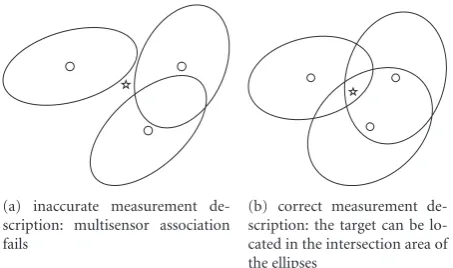
ϕ. The strength of multistatic data fusion is to exploit the inputs from (at least two) source receiver geometries to estimate the targets true position with a higher accuracy, using a kind of triangulation technique by overlaying the uncertain position measurements available. A prerequisite for this triangulation is an unbiased estimation and correctly modelled uncertainties. The difficulty is sketched inFigure 3. Measurements of the same target (star), but corresponding with different illuminator and receiver configurations, are illustrated by their mean (circles) and covariances (ellipses). If the estimate is biased or has an undersized covariance,
Figure 3(a), this may prevent the algorithm from correctly associating measurements of different source-receiver pairs to the same target. For correct measurement modelling,
Figure 3(b), the target can precisely be located in the intersection area of the ellipses.
Additionally, due to item (4) inTable 1and (even worse because of aspect dependency) due to item (6), not only are target echoes fed into the data fusion, but also false alarms. This results in multiple hypotheses for triangulation crossing points, and the correct association between target and received echoes has to be made. This is why estimation errors should not be modelled too pessimistically, since this would lead to too many crossing possibilities.
Again due to items (4) and (6) (Table 1), the detector (i.e., the software that generates contact data) cannot analyze all parts of the signal: A kind of decision threshold has to be defined to set the performance of a specific sensor following its receivers operating characteristics (ROC). This defines the probability of detection (PD) and probability of false alarms (ρF) that has to be expected from this sensor. Since echoes from the target can be missed, the probability for this hypothesis has to be taken into account within all following data fusion and processing steps. Item (5) is increasing this difficulty: due to fading channels, even for a high false alarm setting it is not guaranteed that the target echo has generated a contact.
(a) inaccurate measurement de-scription: multisensor association fails
(b) correct measurement de-scription: the target can be lo-cated in the intersection area of the ellipses
Figure3: Visualisation of multisensor fusion. The measurement information of three S/R pairs is visualized by ellipses. The true target location is shown as a star.
Correct modelling of these probabilistic effects for each single bistatic source and receiver combination is the pre-requisite of multisensor fusion. In the next section, we will show, how it can be handled within the scheme of automatic sequential tracking techniques.
5. Automatic Sequential Tracking Techniques
Bayesian target tracking is iterative updating of conditional probability densities of the target state xk (containing the target components that are to be estimated, for example, the target position and velocity) at timetkgiven all accumulated sensor dataZk = {Z1,. . .,Zk}, whereZk = {zk(1),. . .,zk(nk)} denotes the set of nk measurements collected at time tk. It exploits all available a priori information on the target dynamics and the sensor performance in terms of statistical models. Each update consists of a prediction, which is determined by the target dynamics model. The prediction is followed by a filtering step, which exploits the current sensor data and the sensor model. The sensor data at each scan
k, as well as the sensor model, are the constituents of the likelihood function. According to Bayes’ rule, the conditional density at timetk, given all sensor data up to and including timetkcan be sequentially calculated, that is
pxk|Zk
=pxk|Zk,Zk−1
∝p(Zk|xk)p
xk|Zk−1
, (12)
can be derived from the densities optimal estimators accord-ing to particular cost functions. The likelihood function
p(Zk | xk) can be understood as a weighting function, scoring possible target states by the new incoming data. The likelihood reflects the match of measurement and target state, additionally it depends on the sensor performance. Thus, letek denote the event of target detection by one of the measurements inZk andek be the event that the target was missed, then the single target likelihood function can be separated in two summands
with
p(Zk,ek|xk)=p(ek|xk)p(Zk|xk,ek)
=p(ek|xk)pFA(nk−1)ρFnk−1
nk
i=1
pz(i)|x
k,eik
,
(14)
where eki represents the interpretation that the target was detected by measurementz(i)k and all measurementsz(j)k with
j /=iare false alarms. Due to the assumption that the target is detected by one measurement at most,pFA(nk−1) represents the probability of obtainingnk−1 false measurements andρF is the false alarm density, that is, the probability of obtaining a false alarm at a specific position of the observation area. The second summand is
p(Zk,ek|xk)=1−p(ek|xk)pFA(nk)ρnFk, (15)
that is, all measurements are false.
5.1. Modelling Assumptions of Sequential Target Tracking. In the application of sequential target tracking, the likelihood function needs to be modelled appropriately: in this paper we assume uniformly distributed false alarms; that is, we choose a fixed value of ρF. Thus, the probability pFA(nk) required for (14) and (15) is calculated according to a Poisson distribution with parameterρF, that is, pFA(nk) = e−ρF(ρnk
F /nk!). The probability of detection p(ek | xk) is further replaced by some fixed valuePD. According to these assumptions, the likelihood function can be calculated. But, obviously, the choice of the parameters PD and ρF will have a significant influence on the tracking process. These assumptions on the probability of detection and false alarms are typical for many tracking applications, see for example [1,11]. We will use this by default in our tracking algorithm. InSection 7, we discuss the consequences of the assumption of a fixedPDin the multistatic scenario in more detail and present an approach to mitigate this constraint.
The target motion model is describing the evolution of the target state over time and needs to be defined in the tracking algorithm. We use the nearly constant velocity model that describes evolution by a linear transformation Fk+1|k plus a noise termGk+1|kvk+1 which is modelling the uncertainty about the targets next movement, that is,
xk=qk, ˙qkT, withqk=x,yT and ˙qk=x˙, ˙yT (16)
xk+1=Fk+1|kxk+Gk+1|kvk+1, (17)
whereFk+1|kandGk+1|kare matrices andvk+1is a Gaussian process noise, see [12,13].
5.2. Data Association and Tracking with Multihypothesis Tracking (MHT). In this section, an implementation of automatic sequential tracking is described. The implemented technique is called multihypothesis tracking (MHT). We follow the MHT architecture as described in [13], which will allow us to leverage on it successful application for ground
o z(1)1
z(2)1 o
z(1)2
z(2)2
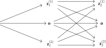
Figure4: Hypothesis generation: In every time scan, the number of hypotheses increases by the factormk+ 1 (number of measurements
plus event of missed detection). A missed detection is illustrated by a circle.
moving target tracking. This section contains only an outline of the implemented MHT, for more details we refer to [13]:
The key idea of MHT is to describe the conditional probability density given in (12) by a Gaussian mixture. Therefore, a hypothesis tree is generated starting from an appropriate initialisation. Every new incoming measurement induces a new hypothesis. As a simple example, we consider a scenario with two measurements at time t1, and also at timet2. After timet1the MHT consists of three hypotheses, either z(1)1 belongs to the target, or z(2)1 , or the target has not been detected. After timet2, the number of hypotheses has increased to 9, as in every time scan the number of hypotheses increases by the factormk+ 1.
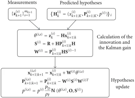
A hypothesis within the MHT tree reflects a specific association possibility and can be represented by an expec-tation,x(i)k+1|k+1, and a covariance matrix,P(i)k+1|k+1(describing a Gaussian density). Additionally, a hypothesis corresponds with a respective weight p(i) that is sequentially updated (Figure 5) and initialized byp(0)=1. For linear dependency of measurement and state vector, that is, zk = Hxk, the Kalman filter formulas can be applied for state estimation. The respective measurement update of each hypothesis is also given in Figure 5. Thus, the MHT consists of several Kalman filters running in parallel, such that its performance depends to a great extent on the performance of the Kalman Filter. For a nonlinear measurement equation (as in multi-static applications), appropriate approximation techniques must be applied. We address this topic in more detail in
Section 6.2.
{H(ki)=(xk(i+1)|K,P(ki+1)|K,p(i))}i Predicted hypotheses
Calculation of the innovation and the Kalman gain Measurements
Hypotheses update {z(ks+1) }mk+1
s=1
θ(i,s)=z(s)
k −Hx(ki+1)|k S(i)=R+HP(ki+1)|kH W(i)=P(i)
k+1|kHS(i)−1
x(ki+1,s)|k+1=x(ki+1) |k+W(i)θ(i,s) Pk(i+1,s)|k+1=Pk(i+1)|k−W(i)S(i)W(i)T
p(i,s)=p(i)PD
ρFN(θ
(i,s),O,S(i))
Figure 5: Measurement update step of the MHT: for each hypothesis H(ki) at time tk and each measurement z(ks+1) a new
hypothesisH(ki+1) =(x (i)
k+1|k,Pk(i+1) |k,p(i)) is generated.
is equal to the sum of hypotheses weights, [13]. Thus, by choosing appropriate thresholdsAandBa track is extracted if the LR exceeds the thresholdAand is terminated if it falls below B. Gating methods ensure individual processing of well separated targets.
Figure 6 illustrates one cycle of the MHT for a single track, it consists of the following steps:
(i) prediction of the current hypothesis tree according to the assumptions on target motion,
(ii) generation of new hypotheses according to the latest measurement information (measurement update, see
Figure 5) and including the possibility of missing detections,
(iii) hypotheses tree reduction techniques,
(iv) evaluation of tracks (confirmation or deletion).
Further instances of track management are track merging and track splitting [13].
6. Approximation Techniques to
Apply Sequential Tracking Techniques
to Multistatic Sonar
By applying the sequential tracking technique, the multistatic measurement is split into bistatic measurements which are fed one by one into the tracking algorithms.
6.1. Handling Large Number of Contacts. For active sonar, as described in Section 2, the target strength of a submarine is designed to be small. As also described inSection 2, the application of active sonar in shallow water produces a large number of false alarms. Using all these contacts would stress the MHT structure and would cause an intractable size of the hypothesis tree. On the other hand, due to the multiple aspects of the target in multistatics, there is a high probability for a strong echo of at least one of the receivers. We are making use of this implicitly by defining an initial threshold
(IT) with contacts whose SNR-value has to cross in order to initiate a new track. The detection threshold (DT) is used for updating existing hypotheses, allowing high accuracy maintenance of the track. The detection threshold (DT) is used for updating existing hypotheses. DT is lower than IT allowing for as many cross-fixing opportunities with contacts from different S/R as possible in order to maintain high accuracy of the target state estimation inside the track.
6.2. Handling Nonlinearities in Target Tracking for Bistatic Sonar. In the application of monostatic and bistatic sonar, the measurements are nonlinear functions of the target statexk and the environmental parametersa =(cS,oT,sT). Ignoring noise effects, the measurement vectorzk(eitherzFMk orzCWk ) can be described by a nonlinear function
zk=h(xk,a). (18)
The functional relationship in h is directly related to the functiong(zFM
k ,a)=q(defined inSection 3). Note thathis not invertible since the dimension ofxkandais larger than the dimension ofzk. Thus,has well asgpresume knowledge ofa.
Several approximation techniques like the EKF [5] and UKF [4] exist and fit perfectly in the framework of the MHT: only the measurement update component (seeFigure 5) of the MHT is affected.
To concentrate on the measurement update and to ignore influences of the MHT approximations, we look in this section at a simplified scenario of one target, one source receiver pair and no missed detections and false alarms. Thus, the MHT structure reduces to a simple Kalman filter that consists of two steps: Prediction of the track state (usually in Cartesian coordinates) and track update using the measurement information. Two different ways to handle the nonlinear measurement equation in these schemes are investigated:
(i) the measurement is transformed into Cartesian coor-dinates and the Kalman Filter updates the target state in Cartesian coordinates (resulting in two algorithms: Cartesian L and Cartesian UT, resp.);
(ii) the predicted state is transformed into the measure-ment space to perform the filter update (which is the method used in UKF and EKF algorithms).
Figure 7illustrates these two approaches.
The application of the Cartesian Kalman Filter works in a straightforward way by exploiting the transformation described inSection 4.1. Instead, the standard UKF and EKF need to be adapted to account for the uncertainties in the environmental parameters. As inSection 4.1, we assume the heading vector to be zero and pick up the uncertainty in the azimuth uncertainty.
Timetk
{H(i)=(x(i)
k|k,P(ki|)k,p(i))}Ni=(1k) Current hypotheses
{H(i)=(x(i)
k+1|k,P(ki+1) |k,p(i))}Ni=(1k) Measurements
{(xk(i+1,s)|k,Pk(i+1,s)|k,p(i,s))}N(k),mk+1
i=1,s=1
Gating ++ pruning ++ merging hypotheses reduction
{H(i)=(x(i)
k+1|k+1,P(ki+1)|k+1,p(i))}Ni=(1k+1) Trackscore=N(k+1)
i=1 p(i)
New hypotheses
Trackscore> A
Track evaluation Trackscore< B
B≤trackscore≤A Prediction
Measurement update Missed detection
Wait
Confirm track Terminate track Timetk+1 {zk(s+1) }ms=k1+1
{(x(kℓ+1)|k,Pk(ℓ+1)|k,p(ℓ)(1−P D))}Nℓ=(k1)
(see Figure 5)
Figure6: One cycle of the MHT: prediction of hypotheses; update of hypotheses; hypotheses reduction (by gating, pruning, and merging); track confirmation or deletion.
of the target statexkat timetkgiven the measurement history,
Zk= {z1,. . .,zk}, and all available a priori information, here
a∼N(a;a,Ca), whereadescribes the assumed values anda the unknown, but true parameters:
pxk|Zk,a
=
pxk,a|Zk−1,zk,a
da
=
pzk|xk,a,Zk−1,apx
k,a|Zk−1,a
p(zk|xk,a)p(xk,a|Zk−1,a)d(xk,a)da
=
Nzk;hx(a)
k
,RNx(a)k ;x(a)k|k−1,P(a)k|k−1
Nzk;h
x(a)k ,RNxk(a);x(a)k|k−1,P(a)k|k−1dx(a)k da
≈
Nzk;Hx(a)
k ,R
Nx(a)k ;x(a)k|k−1,P(a)k|k−1
Nzk;Hx(a)k ,RNx(a)k ;xk(a)|k−1,P(a)k|k−1dx(a)k da
=
Nzk;Hx(a)
k|k−1,S
Nx(a)k ;xk|k−1+W
zk−Hx(a)k|k−1
,P(a)k|k−1−WSW
Nzk;Hx(a)k|k−1,S
Nxk(a);xk|k−1+W
zk−Hxk(a)|k−1
,P(a)k|k−1−WSWdx(a)k da
=
Nxk(a);xk|k−1+W
zk;Hx(a)k|k−1
,P(a)k|k−1−WSWda
(19)
Line 2 of (19) yields due to the Bayes rule. In line 3 we define the extended state vectors byxk(a) =(xk,a)T,x(a)k|k−1 =
(xk|k−1,a)T and state covariance P(a)k|k−1 =
Pk|k−1 O
O Ca
.
Linearization ofh(xak)≈Hxak+b=H1xk+H2a+bdelivers
the approximation in line 4. Line 5 follows from the Gaussian refractorization lemma
N(z;Hx,R)Nx;y,P
whereS=HPHT+R,W=PHTS−1with appropriate vectors and matricesx,y,z H,P,R.
By extending the target state vector, we can apply the standard EKF or UKF formulas to derive x(a)k|k. Since we are not interested in an update of a (it is assumed to be independent for different pings), calculation can be simplified for the EKF:
xk|k=xk|k−1+W1(zk−h(a,xk))
Pk|k=Pk|k−1−W1SWT1,
(21)
where S = H1Pk|k−1HT1 + H2CaHT2 + R, and W1 =
Pk|k−1HT1S−1. Alternatively, we can use the UKF equivalents ofSandW1.
Consequences on the Architecture of the MHT. Due to the nonlinearity in the measurement model, approximation techniques are necessary to apply sequential target tracking to multistatic sonar. Comparing the approximation tech-niques linearization and UT, we find that linearization tends to underestimate the actual errors whilst the UT tends to overestimate, simulation results are presented in
Section 8.2.1. Referring to multistatic tracking performance, the two methods based on UT (Cartesian UT and UKF) seem to be preferable and deliver robust tracking results. The analysis with simulated data leads the choice to the UKF as component of the MHT. We prefer the UKF to the Cartesian UT for two reasons.
(1) The UKF method can easily be extended to process additional Doppler information.
(2) Incorporation of the deterministic features (Section 3) is straightforward in the framework of the UKF.
7. Multisensor Fusion
To exploit information from several source/receiver (S/R) pairs an appropriate strategy for multisensor fusion must be developed.
The next two subsections give details of the implementa-tions of the “AND” and “OR” fusion strategy. Then, in a third subsection we develop a new “adaptive” scheme.
7.1. Implementing “AND” Data Fusion in the Framework of MHT. The “AND” fusion strategy fits perfectly in the idea of the MHT. InFigure 6, a cycle of the standard MHT (used in this work) is illustrated. If measurements ofk S/R pairs and the same time scan are available we can process the information by sequential updating track hypotheses, this is illustrated inFigure 8(a).
It can be shown that (if measurements of different receivers are uncorrelated) sequentially updating of contact information according to the Kalman filter equation is equal to updating the information together. However, as described inSection 5.2, the MHT is based on suboptimal implementation techniques (each measurement update is followed by hypotheses reduction techniques). Thus, in fact, the order of updating may influence the result.
The “AND” rule does not presume that contact informa-tion of every S/R pair is available, rather a track must follow the assumptions aboutPDandρFof each single S/R pair.
7.2. Implementing “OR” Data Fusion in the Framework of MHT. The idea to implement the “OR”-rule is to run a single-sensor MHT tracker first at the data sets generated by each S/R pairs. It has to be pointed out that the overall probability of detection for a single bistatic receiver MHT is lower than for the complete multistatic system as described in Section 6.1. Furthermore, the single bistatic receiver MHT cannot exploit triangulation features as described in
Section 4.2. The measurements associated with the n-best hypotheses are considered for a second MHT chain that runs on the preprocessed data of all S/R pairs. This second MHT follows the same architecture as described in the above subsection, but the two strategies differ with respect to the calculation of the hypotheses weights and therefore in track evaluation. Here, a hypothesis is not penalized for a missing detection as long as the hypothesis coincides with the detection of at least one S/R pair, seeFigure 8(b). The “OR” rule differs from the “AND” rule with respect to the following aspects.
(i) Only measurements associated with an bistatic track are considered in the fusion step.
(ii) A track can be extracted if it follows the assumptions aboutPDandρFof a single S/R pair.
7.3. Situational Adaptive Scheme. Both the “OR” and the “AND” fusion strategies are not perfect. Because in the “OR” fusion strategy the MHTs do not have a direct access to all multistatic contact data, the “OR” results do not fully exploit the multistatic measurement setup. The “AND” fusion is very sensitive with respect to an inadequate measurement modelling that could result in an inadequate description of the measurement error or a bias (see also Section 4.2). Especially, “AND” fusion is sensitive with respect to the assumption of a fixedPD. Let us assume a simple scenario, where there are two receivers, but only one receiver delivers contacts of the target. If the assumed PD is high for both receivers the “AND” fusion strategy will not be able to track the target (since waiting for measurements of the second receiver).
Cartesian KF
Cartesian
Measurement g
UKF/EKF
h
{xk|k−1,Pk|k−1} {xk|k,Pk|k}
{zCk,RC}
{a,Ca}
{zk,R} {xk|k−1,Pk|k−1}
{a,Ca}
{xM
k|k−1,PMk|k−1} {zk,R}
{xk|k,Pk|k}
Figure 7: Track update schemes: Cartesian KF (left): Transformation of measurement zk into Cartesian state; UKF/EKF (right):
Transformation of predicted track state into measurement space.
. . . Prediction
Track evaluation Processing chain (S/R 1)
Processing chain (S/R 2)
processing chain (S/Rk) Contacts (S/R 1)
Contacts (S/R 2)
Contacts (S/Rk)
(a)
. . . .
. . Prediction
Prediction Prediction Processing (S/R 1)
Processing (S/R 2)
Processing (S/Rk) Evaluation
Evaluation
Evaluation
ontacts (S/R 1
C )
Contacts (S/Rk) Bestn
Bestn
Bestn Contacts
Contacts
Contacts
Prediction
Processing chain (S/R 1)
Processing chain (S/R 2)
Processing chain (S/Rk) OR
OR
OR
Track evaluation Contacts (S/R 2)
(b)
Figure8: Visualisation of the “AND” (a) and “OR” (b) fusion strategy. A processing chain in the MHT framework contains updating of hypotheses by available contact information and hypotheses reduction techniques.
in the application to sequential target tracking is to estimate correctly the accuracy of the additional information used.
7.3.1. Sonar Equation. The sonar equation combines in logarithmic units (i.e., units of decibels relative to the standard reference of energy flux density of rms pressure of 1μPa integrated over a period of one second) the following terms:
SNRout=(S−TL1−TL2)−(NL−AG) + TS (22)
which define signal excess where: S: source energy flux density at a range of 1 m from the source; TL: propagation loss for the range separating the source and the target (TL1) and the target and the receiver (TL2); NL: noise energy flux density at the receiving array; AG: array gain that provides a quantitative measure of the coherence of the signal of interest with respect to the coherence of the noise across the receiving array; TS: target strength whose value strongly depends on
the aspect of the target to the source receiver pair, if the target is a long thin cylinder.
For the description of active sonar, the sonar equation has to be applied for the sound path from the source to the target where the received level plus the target strength (TS) is reflected to the receiver. Especially interesting with respect to target tracking are the parts of the sonar equation, which depend on the target position (TL, TS, and NL) and on target position and velocity (TS).
In this paper, we only refer to the sonar equation in the noise limited case, because this is the version used in the algorithms described below. A similar treatment could be proposed for the reverberation limited case.
target-SNR to be Gaussian distributed with a deviationσdB. This is also assumed to be the deviation of the noise level [14]. Then, the probability of detection is a function of the target state and the detection thresholdλand can be obtained by integration
PD(xk,λ)=p(hSNR(xk)> λ)=
∞
t=λN
t;hSNR(xk),σdB2
dt,
(23)
assuming Gaussian distribution. Because PD depends on the target’s location and aspect, which is exactly what a target tracking algorithm provides as prediction, we use the tracking knowledge when calculating the PD value. Therefore, let Bk denote the interpretation of the track history up to time tk; that is,Bk consists of the eventseis, s=1,. . .,k:
es
i=
⎧ ⎨ ⎩
measurementzisbelongs to target ifi /=0
target was not detected at times ifi=0. (24)
For each hypothesis branch of the MHT, we compute the expected probability of target detection ek at timetk given its respective measurement historyBk−1and the hypothesis of target existenceH1. Thus, the weighting of a hypothesis branch is influenced by the modelling of the detection performance
p(ek|Bk−1,H1)=
p(ek,xk|Bk−1,H1)dxk
=
p(ek|xk,Bk−1,H1)p(xk|Bk−1,H1)dxk
= ∞
t=λN
t,hSNR(xk),σdB2
dtNxk;xk|k−1,Pk|k−1
dxk
≈ ∞
t=λN
t−b,Hxk,σdB2
dtNxk;xk|k−1,Pk|k−1
dxk
=
∞
t=λN
t−b,Hxk|k−1,σdB2 +HPk|k−1HT
dt,
(25)
where xk|k−1 and Pk|k−1 denote the estimated target state and covariance respective to the interpretation historyBk−1. Row 4 results from row 3 by linearization of hSNR by hSNR(xk) ≈ b+ Hxk. The last equality holds due to the Gaussian refactorization lemma (20). The first term at row 4 becomes independent of the target state xk whilst the second term is a probability density ofxk, thus the integral is 1.
The pdf is a function of the predicted target state and of the accuracy in this estimate. Thus, the considered Gaussian density becomes flatter with decreasing knowledge about the target state. In the limiting case, the probability is.5.
Usually, the functional relationship in hSNR cannot be described by a simple function. Noise measurements in each bearing and for each receiver and the output of target strength and propagation loss modelling software are used to calculate the actual value of hSNR(xk). Since the derivation, presented above, utilizes the linearization of hSNR, we would need to calculate the derivatives of hSNR with respect to the target state components. How-ever, hSNR is generally a strongly nonlinear function, thus the linearization may be problematic. Replacing the lin-earization by UT to derive HPk|k−1HT makes it possi-ble to apply the approach without looking deeper into the function hSNR; thus, we can even process tabular entries.
7.4. Fusion of FM and CW Contacts. During the experiments with the deployable multistatic sonar systems, FM and CW signals were transmitted simultaneously. In this case, when regarding to the same target, source and receiver geometry, the values for TL, TS, and NL are quite comparable for both signals. Thus, fusion of FM and CW contacts according to the “AND” rule seems to be straightforward. We can exploit these geometrical similarities but need to consider some differences resulting from the types of signals. Whilst with FM a good range resolution is obtained, the CW delivers additional Doppler information, but with lower range resolution. As a consequence of the poor resolution in range, we decided that CW contacts will not be used for track initialisation. Furthermore, the probability of detection (PD) of a CW measurement is not only dependent on the SNR of the target (Section 7.3), but is additionally dependent on the measured Doppler value [2]. If the Doppler of the target is close to the Doppler of the background, the target is in the so-called clutter notch and the probability of detection is low. The eventuality that a target is in the Clutter notch does not only concern nonmoving targets, but may also appear due to geometrical reasons. In particular, in bistatic applications, these geometrical clutter notches take shape [15] and make demands on regarding to the phenomena of the clutter notch. Let ˙rT be the range rate of the target and ˙rC the range rate of the corresponding background. Using the modelling assumption in [2], we express the PD depending on the distancenC(xk) = |r˙T −
˙
rC|, on a characteristic sensor information, the minimum detectable velocity (MDV), and a part pD(xk), that can either be chosen to be fixed or SNR adaptive (see [2] for details)
PD(xk)=pD
1−exp
−ln(2) |r˙
T−r˙C|
MDV
2
=pD
1−MDV
ln(2)/πN
0;nC(xk), MDV2 2 ln(2)
.
(26)
p(ek|Bk,H1)=
p(ek,xk|Bk−1,H1)dxk
=
p(ek|xk,Bk−1,H1)p(xk|Bk−1,H1)dxk
=
pD
1−MDV
ln(2)/πN
0;nC(xk), MDV2 2 ln(2)
Nxk;xk|k−1,Pk,k−1
dxk
≈pD
1−MDV
ln(2)/πN
−b;NCxk|k−1,MDV 2
2 ln(2)+NCPk|k−1N T C
.
(27)
From row three to four, we exploit the Gaussian refac-torization lemma and a approximation by linearization of
nC(xk) = b +NCxk. The derivation shows that only the predicted state estimate and state covariance influences the considered probability of detection.
For the fusion step the CW contacts are similarly processed to FM contacts. But the modelling assumption of thePD (26) will have influence on hypothesis weighting and even on the track update process. The update formulas are derived according to the Bayes formalism in [2]. As it can be seen in (26) the fictitious “measurement” that the target is in the clutter notch, is Gaussian distributed due to the modelling assumptions and can therefore be processed as an additional “measurement” information. The EKF approximation (utilized in [2]) is again replaced by an UKF approach, see [15]. The fusion of CW and FM contacts is an example for a situational adaptive fusion scheme as motivated in Section 7.3. A priori knowledge about the clutter notch is imbedded in the tracking algorithm. But, the fusion of FM and CW goes even one step further by defining the fictitious “measurement”. For the situational adaptive scheme presented inSection 7.3, only hypothesis weighting but not state estimation is influenced.
The “AND”, “OR”, and situational adaptive fusion of measurements of different S/R pairs can easily be adapted to account for additional CW contacts.
For the “AND” fusion strategy, the consideration of CW contacts is straightforward; all available contact files (FM and CW contacts) are exploited for sequentially updating the hypothesis tree (regarding to the characteristics of the CW signal); we later refer to this as “AND” fusion strategy of FM and CW contacts.
Similarly, the “situational adaptive fusion of FM and CW contacts” is straightforward. The fixedPDsettings for the FM and the fixed part of thePD for the CW will be estimated from the sonar equation.
The “OR” fusion strategy is adapted to combine FM and CW contacts in the following way (later to be referred to as “OR” fusion strategy of FM and CW contacts):
(i) tracking of FM and CW contacts of each S/R pairs (“AND” fusion of FM and CW contacts);
(ii) taking the FM contacts associated to tracks and running a second instance of the MHT.
Interesting with respect to the phenomena of the clutter notch in multistatic sonar are nonmoving targets such as a wreck. Wrecks produce continuous FM contacts, whilst they are not detected by the CW signal. This is different in typical scenarios of ground moving target tracking and allows a look at the phenomena of the Clutter notch from a different point of view. We will discuss results inSection 8.1.4.
8. Data Analysis
In the previous sections, many adaptations of the MHT structure have been developed. In this section, we demon-strate the necessity for making these amendments. There are several data sets from measurements at sea available. We apply them to the derived algorithms, stepwise increasing the level of precision of the sensor modelling. We show that the tracking performance increases when correctly modelled details of the sensor model are added. In its final state, the algorithm is able to deliver high precision target state information and a very low false alarm rate. However, measurement at sea is cost and time intensive. Not all statistical aspects of the algorithm’s design can be significantly answered by the limited data set. Therefore, we augment the experimental data by numerical simulations in order to evaluate the different possibilities for necessary numerical approximations inside the tracking process. We will also see an example for the necessity to improve the motion model: since our motion model does not include possible turns and since inside the tracking algorithm only small uncertainties due to precise modelling exists, strong manoeuvres of the target seem to decrease the quality of the performance of the tracker with the better sensor model, see
Section 8.1.4(a). We propose to rather improve the motion model, see for example [16], instead of arguing for a more robust, but imprecise sensor model.
8.1. Data Analysis with Experimental Multistatic Sonar Data.
In this section, we test the different adaptations of the MHT algorithm. Table 2 provides an overview of the different modes and specifies the section of more detailed informa-tion.
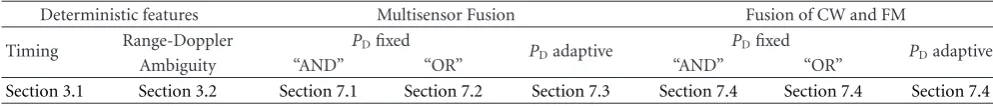
Table2: Overview of different versions of the multistatic MHT.
Deterministic features Multisensor Fusion Fusion of CW and FM
Timing Range-Doppler PDfixed PDadaptive PDfixed PDadaptive
Ambiguity “AND” “OR” “AND” “OR”
Section 3.1 Section 3.2 Section 7.1 Section 7.2 Section 7.3 Section 7.4 Section 7.4 Section 7.4
when correction for timing and Range/Doppler ambiguity is applied simultaneously), (3) “AND” fusion of FM, (4) “OR” fusion of FM, (5) adaptive fusion of FM, (6) “AND” fusion of FM and CW, (7) “OR” fusion of FM and CW, and (8) adaptive fusion of FM and CW. The measurement update step is always realised by the UKF as motivated inSection 6.2. Unless specified otherwise the different fusion strategies are applied in combination with the DoTiCor approach.
8.1.1. Description of the Data Sets. In the course of NURC’s project on deployable multistatic active sonar, two major sea trials were conducted: PreDEMUS’06 and SEABAR 07. Measurements at sea have been executed within the Scientific Program of Work at the NATO Undersea Research Centre (NURC). Since the data have been distributed among several research institutions in NATO, we use the original names given to the data sets for potential further reference.
Note. Experiments at sea generate only a limited set of data and are conducted under specific equipment and safety constraints. For further sensitivity studies and specific statistical performance analysis we added simulated data sets;
Section 8.2.
Common to all data sets is the usage of the deployable buoy system (Figure 1, called DEMUS).
(i)DEMUS Receivers.The systems are built on a frame of 9 arms; each arm is made up of 7 acoustic outputs or staves. Each of these acoustic outputs is produced by summing three vertical hydrophones. The lateral spacing of hydrophones is variable and can be set remotely. The system is designed to operate in the range 2–5 kHz. The level of the “Input Referred Noise” across the band of interest is lower than the noise level at calm seas, making the receiver a high-quality measurement system. The system is bottom tethered, typically at 100 m depth. Nonacoustic output of the system contains of depth, compass, and tilt.
(ii)DEMUS Transmitter. The transmitter is tethered in the same way as the receiver. The operating frequency range is 2–4.2 kHz. It is constructed from 8 FFRs, where weightings can be applied to outputs for vertical steering and beam shaping. The typical battery life is 500 ping seconds.
Also, common to all data sets is that an artificial target was used, called echo-repeater (or E/R). The E/R was towed by a surface vessel at a depth of 80 m. It retransmits received source signals with a specified amplification (TSER) and a certain delay. For the delay, the contact data have been
already corrected. Details of this correction process are omitted here, but it is obvious that a high TSERlevel is needed to identify uniquely the corresponding contacts. Resulting received signal-to-noise ratios (SNR) are unrealistically high, but can be decreased by simply inserting lower values in the corresponding data structure of a contact [17]. However, with this procedure it is possible to generate contacts for the target that in a real scenario would not occur because their SNR would correspond to a threshold setting for contact generation that is too low.
For data analysis, we consider five data sets based on PreDEMUS’06 B01, SEABAR 07 A01, and A56:
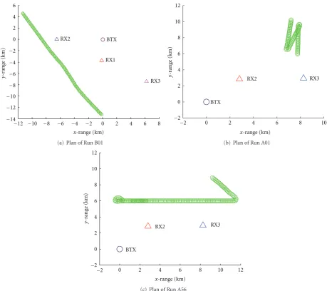
(a) PreDEMUS’06 B01. The setup of PreDEMSUS’06 is shown inFigure 9(a), a single source and three receivers were installed. E/R signals are detected within a moderate noise background generated by distant shipping. DT and IT are set to 10 dB for FM contacts. CW contacts are all taken without a threshold. The corresponding input files for each source receiver pair contain about 60 contacts per ping for FM and about 90 contacts per ping for CW.
(b)SEABAR 07 A01 50. The setup is shown inFigure 9(b), detections of two receivers and one source are given. E/R signals are detected within a high reverberation level plus time-varying directional high noise levels from close shipping. The data set contains the best 50 contacts of the FM processing and all (about 100) contacts from the CW processing. IT is set to 10 dB.
(c) SEABAR 07 A01 TS. As in SEABAR 07 A01 50 and A01 10dB, but now the SNR values of the target contacts have been reduced [17]. The tracker has to process about 500 contacts per ping and each S/R pair for the FM and again about 100 contacts for the CW. A threshold of 2 dB is set to the reduced E/R contacts causing a reasonable number of missed detections. The IT was again 10 dB.
(d)SEABAR 07 A56 50. The setup is shown inFigure 9(c), detections of two receivers and one source are given. During Run A56, the measurement was made in bad weather conditions. We use the time synchronized data set, but with the original target SNRs [17]. It contains the best 50 contacts of the FM processing and all contacts from the CW processing (about 100). IT is set to 10 dB.
8.1.2. Performance Metrics. In the following, we will assess the performance of the proposed extensions by applying the different modes of the algorithms to these data sets. Changes in performance should be made visible when calculating measures like track duration, track fragmentation, latency,
false track rate, andestimation performance. We will corre-spond to track duration, latency, and track fragmentation by indicating the time of track extraction (TE) and termination (TT). Thus, the track latency corresponds to the TE time; the track duration can be calculated by (TT-TE), and track fragmentation is demonstrated by indication of several times of TT and TE. This is different from the track duration metric defined in [18], which counts for the measurement associations since initialization of a tentative track.
The total track rate (mean number of tracks per ping) that is utilized in this paper counts for all extracted tracks (including the true target track), it is directly related to the false track rate.
Estimation performance is either specified by calculating the estimation errors or illustrated by direct comparison of target and track trajectory.
8.1.3. Results for PreDEMUS’06 B01. The data set B01 was analysed by detailed postprocessing to determine the exact position of the E/R sound source, thus quite accurate truth information is available.
(a) Impact of Deterministic Features—SEABAR 07 A01 50 and SEABAR 07 A01 10 dB. The algorithms DoCor, TiCor, and DoTiCor, as defined inSection 3are applied and their performance is compared to the versions without correction (NoCor). All results correspond to fusion of FM contacts of RX1, RX2 and RX3 according to the “AND” fusion strategy (CW measurements are not considered). InFigure 10(a), the estimation error of the algorithms is plotted, demonstrating that the corrections are necessary.Figure 10(b)demonstrates this by plotting the results of the DoTiCor and NoCor approach in the 2D plane. Results for the correction of the Doppler ambiguity are shifted. The bias in the range measurement due to the frequency shift is compensated.
Remark. The effect of the corrections depends on the given geometry.
(b)Results of Different Fusion Strategies—PreDEMUS’06 B01.
Within the noise background and the chosen false alarm rate, detections from receiver RX1 and RX3 are not possible due to the large distance to the target for the first 50 pings, see
Figure 11. Clearly, the “AND” strategy suffers from missing detections in at least a second receiver. Close to ping 30, detection was missed for all three receivers for about 10–20 pings. After that the target is quite frequently detected by all three receivers.
Following the description of the fusion strategies in
Section 7 we apply the different fusion approaches to the data set of PreDEMUS’06 B01 (all utilizing the DoTiCor approach). Results are shown inTable 3.
The missed detections of RX1 and RX3 in the beginning affect the tracking results. Thus, when pursuing the “AND” fusion strategy (1st row), the target track is not extracted in an initial phase of about 50 pings. As expected, the “OR” fusion strategy (2nd row) gives better results in this region, since contact information of RX2 is sufficient for track extraction.
For the situational adaptive scheme (3rd row), the values for TL were calculated according to the distance between source, receiver, and estimated target state. The NL level was fixed (assuming a stationary noise background) and since an E/R does not have aspect-dependent target strength, the TS value was also kept constant. In the considered scenario the situational adaptive scheme proves to be an adequate compromise between “AND” and “OR” fusion strategy, it provides good track duration and low false track rate. For both approaches, “OR” fusion and situational adaptive, track fragmentation occurs at ping 28; this is when all three S/R pairs miss detections.
The combination of FM and CW contacts (4th row) results in a significant reduction of false tracks. Additionally, comparison of only FM (1st row) and FM and CW (4th row) shows improvements with respect to track latency, when processing the CW contacts.
Estimation performance was quite comparable for all approaches.
8.1.4. Results for SEABAR A01 50. For the data from A01 only positional information about the E/R towing vessel were available. Thus the E/R (the target) is located behind the position of the vessel depended on the length of the cable. To prevent incorrect estimation of the E/R position we compare our results with the position of the towing vessel.
(a) Impact of Deterministic Features—SEABAR 07 A01 50.
Comparing the results of the DoTiCor approach and the uncorrected version of the MHT (NoCor), we observe an offset in Cartesian estimates, as also noted for PreDEMUS’06 B01. Unfortunately, improvements in localization error can not be verified due to inaccuracies of the truth information. This has be discussed in more detail in [19], it was shown that the application of the DoTiCor approach additional causes degrading tracking performance (from which the MHT can recover) during the first target manoeuvre. The approach seems to be less robust against deviations from the motion model. This is a consequence of the influence that the estimated Doppler has on the range measurement.
(b) Results of Fusion Strategies—SEABAR A01 50. In