Massively Parallel Quantization Implementation
Using Simulated Annealing
by
L. van Engelen
Supervisors:
Dr. Ir. G.J.M. Smit (University of Twente) Ir. E. Molenkamp (University of Twente) Ir. J.W.M. Jacobs (Oc´e)
Drs. Z. Goey (Oc´e)
July 2006 University of Twente
Abstract
This thesis treats the mapping of a quantization algorithm on the Linedancer parallel processor architecture which was done at Oc´e. This algorithm is based on Simulated Annealing and uses a Markov Random Field image model. The mapping of the algorithm was supported by the use of the Evolutionary Design methodology.
The mapping of the algorithm was finished successfully, although the output quality was worse than that of established algorithms. Throughout development an executable prototype was used to guard the quality of the mapping. We identified four typical subphases in the top down part of the Evolutionary Design methodology.
The implementation of the quantization algorithm benefits from the imple-mentation on the Linedancer, demonstrated by a higher processing speed when compared with a Pentium.
2.1 Typical office scan: text and charts. . . 13
2.2 Image degradation: instead of just a couple of solid gray values, the image is blurry and displays some sort of patchwork pattern. The original image consisted of only 10 different grays, but scanning has increased this to 229. 14 2.3 ProbabilitiesP(ys|gs) for the case of quantization to 4 different classes (N = 4). 15 2.4 Approximation of a discrete probabilityP(X =a) based on the continuous probability distributionp(x). 15 2.5 Examples of images of low and high regularity. . . 16
2.6 Image pixel (the black dot) with its neighborhood (gray dots) and corresponding setC of clique pairs. Each clique has its own color. 16 2.7 Fidelity and regularity examples. . . 18
2.8 Acceptance probability at different temperatures. . . 20
3.1 Path of evolutionary design through the design space. . . 25
3.2 Transformational development . . . 26
3.3 Overview of Evolutionary Design: (Sub)phases are passed through from left to right in time. The nesting of the different subphases are also shown. 26 3.4 Increasing portability by using common code templates. Algorithms are implemented in terms of these code templates. For each code template there is an implementation on each architecture. 29 4.1 Expanding a mesh (a) requires more Processor Elements (PEs) than expanding a string (b). 32 4.2 Transfers inside the memory hierarchy of the Linedancer . . . 33
4.3 Associative memory in action. . . 35
4.4 Dependency of the number of cycles on the operand width for the RTS(Mult) and RTS(Div) instructions. 39 4.5 Dependency of the number of cycles on the operand width for the remote RTS(Assign) instruction. 39 5.1 Tiling: the input image is cut into blocks fitting inside the Linedancer and processed in sequence by the Simulated Annealing algorithm. 42 5.2 A 10 bits wide Linear Feedback Shift Register. A 0 is shifted out and 1 Xor 0 = 1 is shifted in. 43 6.1 Comparison of quantizations by (a) a commercial program (Irfanview) and (b) our algorithm. 51 6.2 Tiling artifact in the output of the quantization algorithm. If you look close inside the red rectangle you can see that the blobs have horizontal and vertical borders. These are the tile edges. 53 6.3 Speedup for various image sizes and number of annealing loops. . 54
List of Tables
4.1 Processor Architecture Taxonomy according to Flynn. . . 30 4.2 Some of the RTS instructions that can be used on the Linedancer. 36 4.3 Linedancer operations running with a constant number of cycles. 37 4.4 Linedancer operations which are linearly dependent on the bit width. 38
6.1 Number of cycles used for each stage of the algorithm. Nesting indicates loops, bold numbers indicate accumulated results. 52
6.2 Processing time of Data Stream Manager (DSM) and Instruction Stream Manager (ISM) threads per tile when one annealing loop is performed. 52 6.3 Processing time of DSM and ISM threads per tile when ten Simulated Annealing loops are performed. 54
6.4 Running times of the quantization algorithm on a Pentium and on the Linedancer. 55
A.1 J’s arithmetic and comparison verbs, together with their equivalents in C and mathematical notation. 65 A.2 Operations on whole arrays. . . 65
A.3 Miscellaneous verbs. . . 66
1 Simulated annealing . . . 19 2 Modified Metropolis Dynamics . . . 21
Notation
S Set of all pixels in an image. s Pixel in an image.
g Quantized image.
gs Value of pixelsin quantized imageg. µ Mean value.
µgs Mean value of input image pixels with labelgs.
σ Standard deviation.
σgs Standard deviation of input image pixels with labelgs.
y Input image.
y, ys Value of pixelsin input imagey.
δ(gs, gr) Function returning−1 ifgsequals gr, 1 otherwise. [0,1) Range of real numbers from 0 inclusive to 1 not inclusive.
ALU Arithmetic & Logic Unit: part of a computer processor performing arithmetic and logical functions.
APL A Programming Language: programming language developed by K.E. Iverson, predecessor of J.
CADTES Computer Architecture Design & Test for Embedded Systems: Research group of the Faculty of Computer Science and the Faculty of Electrical Engineering of the University of Twente in the
Netherlands.
CAM Content Addressable Memory: PE memory addressable by its contents instead of a fixed address.
DSM Data Stream Manager: Linedancer thread responsible for transferring data between SDS and PDS.
EXT Extended Memory: Non-content addressable part of the PE memory (cf. CAM).
FPGA Field Programmable Gate Array: Hardware which is reprogrammable at gate level.
GPP General Purpose Processor: A processor which can be used for arbitrary tasks, such as a Pentium.
IDSM Instruction and Data Stream Manager: Processor on which the DSM and ISM threads run.
ISM Instruction Stream Manager: Linedancer thread responsible for controlling the processor array.
LFSR Linear Feedback Shift Register: Shift register which can be used as a semi-random number generator.
MIMD Multiple Instruction Multiple Data: Parallel computing, where multiple instructions operate on vectors of data in parallel. MISD Multiple Instruction Single Data: Parallel computing, where
multiple instructions operate on a single piece of data.
MMD Modified Metropolis Dynamics: parallel optimization of Simulated Annealing.
LIST OF ALGORITHMS 7
MRF Markov Random Field: Field over sets of random variables, with neighborhood relations.
PDS Primary Data Store: Memory used as a buffer for transfers between SDS and PE memory.
PE Processor Element: Single CPU of a massively parallel processor array.
SCC System Control Computer: Aspex’s name for the host CPU of the Linedancer, usually a Pentium.
SDMC Secondary Data Movement Controller: Controller responsible for the transfer between SDS and PDS.
SDS Secondary Data Store: Memory available to the IDSM processor. SIMD Single Instruction Multiple Data: Parallel computing, where one
instruction operates on a vector of data.
SISD Single Instruction Single Data: Nonparallel computing, where one instruction operates on a scalar.
TDS Tertiary Data Store: Memory available to the SCC processor. VHDL Very-High-Speed Integrated Circuit Hardware Description
1 Introduction 11
1.1 Research Question . . . 11
1.2 Overview . . . 12
2 Quantization 13 2.1 Image Model . . . 14
2.1.1 Fidelity . . . 14
2.1.2 Regularity . . . 16
2.1.3 Bayesian Model . . . 17
2.2 Simulated Annealing . . . 19
2.3 Modified Metropolis Dynamics . . . 20
2.4 Choosing Parameters . . . 21
3 Evolutionary Design 22 3.1 Current Practice . . . 22
3.1.1 Oc´e . . . 22
3.1.2 CADTES Group . . . 22
3.2 Alternatives . . . 23
3.2.1 Blaauw and Brooks . . . 23
3.2.2 Bernecky . . . 24
3.3 Evolutionary Design . . . 25
3.3.1 Incremental Prototyping . . . 25
3.3.2 Transformational Development . . . 26
3.4 Intended Benefits . . . 28
3.4.1 Higher Productivity . . . 28
3.4.2 Error Recovery . . . 28
3.4.3 Portability . . . 29
3.4.4 Domain Expert Programming . . . 29
4 Linedancer 30 4.1 Parallel Architectures . . . 30
4.1.1 Processor Architecture Taxonomy . . . 30
4.1.2 Benefits of Parallel Architectures . . . 31
4.2 Hardware Architecture . . . 32
4.2.1 Scalability . . . 32
4.2.2 Memory Transfers . . . 32
4.2.3 Associativity . . . 34
4.2.4 Communication . . . 34
CONTENTS 9
4.2.5 Segmentation . . . 34
4.2.6 Arithmetical and Logical Operations . . . 36
4.3 Programmer’s Interface . . . 36
4.3.1 Software Tools . . . 36
4.3.2 Threads of Execution . . . 36
4.3.3 Libraries . . . 37
4.4 Performance . . . 37
4.4.1 Constant Time Instructions . . . 37
4.4.2 Linear Time Instructions . . . 37
4.4.3 Slow Instructions . . . 38
5 Implementation 40 5.1 Preparation . . . 40
5.2 Incremental Prototyping . . . 41
5.3 Transformational Development . . . 41
5.3.1 Trade-Off Subphase . . . 41
5.3.2 Reorganization Subphase . . . 44
5.3.3 Template Subphase . . . 46
5.3.4 Translation Subphase . . . 49
6 Evaluation 51 6.1 Quantization . . . 51
6.1.1 Algorithm Load Distribution . . . 51
6.1.2 Algorithm Output Quality . . . 51
6.1.3 Performance Analysis . . . 52
6.1.4 Speedup . . . 54
6.2 Methodology . . . 56
6.2.1 Design and Development . . . 56
6.2.2 The J Language . . . 56
6.3 Hardware . . . 56
6.4 Possible Enhancements . . . 57
6.4.1 Algorithm . . . 57
6.4.2 Hardware . . . 58
7 Conclusions and Recommendations 59 7.1 Mapping and Methodology . . . 59
7.2 Quantization . . . 59
7.3 Linedancer . . . 60
A Introduction to J 63 A.1 Comments . . . 63
A.2 Verbs and Nouns . . . 63
A.2.1 Verbs . . . 63
A.2.2 Nouns . . . 64
A.3 Assignment . . . 64
A.4 Arithmetic and Comparison . . . 64
A.5 Array Operations . . . 65
B Listings 67
B.1 Models . . . 67
B.1.1 File: functional.ijs . . . 67
B.1.2 File: functional4.ijs . . . 68
B.1.3 File: functional6.ijs . . . 69
B.1.4 File: algorithm6.ijs . . . 69
B.1.5 File: algorithm9.ijs . . . 71
B.1.6 File: architecture15.ijs . . . 72
B.1.7 File: architecture21.ijs . . . 74
B.1.8 File: templates2.ijs . . . 76
B.2 Linedancer Code . . . 82
B.2.1 File: algorithm.defs . . . 82
B.2.2 File: algorithm.tpl. . . 82
B.2.3 File: ismCode.tpl . . . 86
B.2.4 File: dsmCode.c . . . 86
B.2.5 File: sccCode.tpl . . . 87
B.3 Python Code . . . 88
B.3.1 Parser . . . 88
Chapter 1
Introduction
Oc´e is a manufacturer of printers, copiers, scanners and software and a lot of its technology makes heavy use of image processing algorithms. These algorithms are often of a highly parallel nature, e.g. when they perform the same operation on all pixels of a scan.
Currently, these parallel image processing algorithms are prototyped in a sequential language and finally implemented in a parallel one. This is rather awkward, because when implementing the sequential prototype for a parallel problem a lot of design decisions are taken, so the developer looses a lot of freedom.
One solution to this problem is to use hardware which can be programmed in a language more close to the prototyping language. In order to research this possibility, a massively parallel hardware architecture, called the Linedancer, was introduced.
Although the Linedancer is a parallel architecture and thus lies conceptually close to Oc´e’s typical problems and algorithms, there still is a semantic gap between the prototype and the final implementation. To overcome this problem, a design methodology is researched, called Evolutionary Design.
Our research is focused on understanding the mapping of a parallel image processing algorithm on the Linedancer, with the help of the Evolutionary De-sign methodology. We needed an application and an algorithm as a test case for this mapping process, which would ideally also be of interest to Oc´e. Finally we decided to use image quantization as our problem to solve on the hardware, using an algorithm based on Simulated Annealing and using a Markov Random Field image model.
1.1
Research Question
From the previous we formulate the following research question:
How to map a quantization algorithm, based on Simulated Annealing and using a Markov Random Field (MRF) image model, onto the Linedancer.
We make this research question more concrete with the following subquestions:
• Which problems do we face in mapping the algorithm and how do we face them?
• How does the Evolutionary Design methodology help us during develop-ment?
• How does the Linedancer compare with a General Purpose Processor? • How does the quality of our quantization algorithm compare with
estab-lished algorithms?
During our research our main focus is on the mapping, the image quality produced by the algorithm is of less importance.
1.2
Overview
Here follows a short summary of the structure of the following chapters. In Chapter 2 we introduce the theoretical concepts that lie at the base of our quantization algorithm. We give a mathematical description of our image model and show the algorithm which is based on Simulated Annealing.
In Chapter 3 we give a short summary of current design practices based on the situations at Oc´e and the CADTES research group. We evaluate their benefits and negative sides and introduce the design methodology we used during the implementation of the quantization algorithm.
In Chapter 4 we introduce the hardware we used to implement the quanti-zation algorithm: the Aspex Linedancer massively parallel processor array. The special characteristics of this architecture, such as its associative memory are highlighted.
In Chapter 5 we show how the theories, ideas and technology introduced in the previous chapters are used to implement the quantization algorithm. The methodology is used as the guiding principle through the design space.
Chapter 2
Quantization
Images scanned in an office environment, such as presentation sheets and charts, often contain a limited number of colors (Figure 2.1). During scanning these get distorted. One of the possible distortions is blurring, with the effect that more colors are used in a scan than necessary (Figure 2.2). Reducing the number of colors in such scans can be useful as a first step in image compression. This process is called color quantization. Popular quantization algorithms include the median cut and octree algorithms [12]. These algorithms use a statistical approach: they count the occurrences of each color and try to assign quantized colors using only this information.
We have used the problem of color quantization as a test case for mapping an image processing algorithm on the Linedancer and developing our design methodology. However, to reduce complexity, we quantized grayscale images instead of colored ones. Our algorithm tries to incorporate pixel location infor-mation, in contrast with the aforementioned algorithms.
Figure 2.1: Typical office scan: text and charts. [Typical office scan]
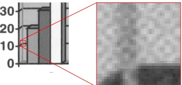
Figure 2.2: Image degradation: instead of just a couple of solid gray values, the image is blurry and displays some sort of patchwork pattern. The original image consisted of only 10 different grays, but scanning has increased this to 229.
2.1
Image Model
In the following we assume that the original input image consists of pixels, each having a gray value of between 0 and 255 and that we want to quantize this image toN different colors. This can be interpreted as the assignment of image pixels toN different classes.
2.1.1
Fidelity
Assume that the pixel values are continuous and normally distributed. This is a common assumption in image processing [7]. The normal distribution has the following form (µandσ are the mean and standard deviation of the distribution respectively):
p(x) =√1 2πσ exp
−(x−µ)2 2σ2
dx, (2.1)
If we know the image pixel value means and standard deviations for each class we can calculate the probability of a pixelswith valueys∈[a, b) belonging to a classgsusing
P(a≤ys< b|gs) =
Z b
a 1 √
2πσgs
exp
−(ys−µgs)
2
2σgs
2
dys, (2.2)
whereµgs andσgs are the mean and standard deviation of pixel values in class
gsrespectively (Figure 2.3). Because pixel values are actually discrete, we define the probability of a certain pixel value ys in the discrete case as the weight of the distribution in a neighborhood of width 1 aroundysin the continuous case. In other words, we define it as probability of the pixel having a value between ys−1
2 and ys+ 1
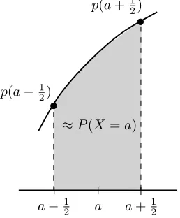
2. From Figure 2.4 it can be seen that we can approximate the discretized probability with the derivative at ys, which simply removes the integral from (2.2):
P(ys|gs) = √ 1 2πσgs
exp
−(ys−µgs)
2
2σgs
2
2.1. IMAGE MODEL 15
0 0
∞
µ4255
µ3
µ2
µ1
P
(
ys
|
gs
)
gs= 1
gs= 2
gs= 3
gs= 4
Pixel value (a) No degradation
0.018
0
ys µ3 µ4
µ2
µ1 255
0
P
(
ys
|
gs
)
Pixel value
σ3
gs= 1
gs= 2
gs= 3
gs= 4
(b) Normally distributed degradation
Figure 2.3: Probabilities P(ys|gs) for the case of quantization to 4 different classes (N = 4).
p(a−12)
≈P(X =a)
a+1 2 a
a−1 2
p(a+12)
(a) Irregular image (b) Regular image
Figure 2.5: Examples of images of low and high regularity.
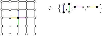
, , , o
C=n
Figure 2.6: Image pixel (the black dot) with its neighborhood (gray dots) and corresponding setC of clique pairs. Each clique has its own color.
We assume that the relation between input image and quantized image only affects corresponding pixels, which means that [10]
P(y|g) =Y s∈S
P(ys|gs). (2.4)
This probability represents the concept offidelity, i.e. the property of the quan-tized image that it resembles the original input image. It gives us a way to compare different quantizations by comparing probabilities. The higher the probabilityP(y|g), the better the quantization matches the original input.
2.1.2
Regularity
While fidelity accounts for the quantization quality of a single pixel, another property called theregularity measures the coherence between quantized pixels (Figure 2.5). This is a property of the quantized result, which is assumed as prior information. Because we focus our algorithm on business graphics we assume that the results consist of connected regions of the same color, called blobs.
To incorporate this into our model we make use of a MRF model. In this model, the value of each quantized pixel only depends on itsneighborhood. These dependencies are called thelocal characteristics of the MRF. Sets of pixels that are all neighbors of each other are calledcliques and the set of all cliquesC in the entire image is denotedC (Figure 2.6).
2.1. IMAGE MODEL 17
joint probability in the form
P(g) = 1 Z exp −E(g) ˆ T , (2.5)
whereE(g) encodes the local characteristics. ˆT is a constant called the temper-ature after its meaning in statistical physics from which (2.5) originates. Z is a normalization constant, to make sureP(g) is a real probability.
Theenergy,
E(g) =X C∈C
VC(g), (2.6)
is built up by theclique potentials VC(g). These are functions defined for each clique and only depend on the pixels inside this clique. So, it is possible to model the joint probabilityP(g) with clique potentials instead of local charac-teristics. In our case we only use the cliques C which are pairs (s, r) and all clique potentials are the same:
VC(g) =V(s,r)(g) =δ(gs, gr). (2.7) The δ(gs, gr) function returns −1 if gs equals gr, +1 otherwise. So, similar pixels pairs contribute−1 to the energy, the others contribute +1.
Combining (2.5), (2.6) and (2.7) we finally arrive at:
P(g) = 1 Zexp
−1
ˆ T X (s,r)∈C2 δ(gs, gr)
. (2.8)
Here,C2 is the set of all pair cliques.
2.1.3
Bayesian Model
To give an idea of the terms fidelity and regularity, Figure 2.7 shows two cases. We can interpret the (normalized) fidelity and regularity as probabilities: let P(y|g) be the fidelity (i.e. the probability of observing input image y wheng is the quantized image), and P(g) be the regularity (i.e. the probability of g being a satisfying quantized image). Using Bayes law [15]
P(g|y) =P(y|g)P(g)
P(y) , (2.9)
which can now be interpreted as the probability of g being the original image when image y is observed, we obtain a measure of the suitability of an quan-tization given an input image in terms of the fidelity and regularity. To find the quantized image given our input we have to maximizeP(g|y), theposterior distribution. Theevidence, P(y) is constant for giveny, so this term can be ignored for the maximization.
We now explicitly derive the expression that we want to maximize, using (2.4) and (2.8):
P(y|g)P(g) =Y s∈S
P(ys|gs)1 Z exp
−1
ˆ T X (s,r)∈C2 δ(gs, gr) = 1 Zexp X
s∈S
−ln√2πσgs−
(ys−µgs)
2
2σ2 gs
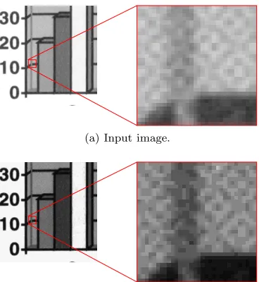
(a) Input image.
(b) High fidelity, low regularity: result looks like the original, but does not have connected regions.
(c) High regularity, low fidelity: result has con-nected regions but looks less like the original.
2.2. SIMULATED ANNEALING 19
BecauseZ−1 is constant and logarithms are strictly increasing, we can take the logarithm of (2.10) and optimize that instead. We also useβ = ˆT−1 to denote the inverse temperature from here on. Finally we can take out a negative sign and minimize the following:
E(g) =X s∈S
ln√2πσgs+
(ys−µgs)
2
2σ2 gs
| {z }
fidelity
+βX C∈C
δ(gs, gr)
| {z }
regularity
. (2.11)
From this we can see that β determines the relative weight between fidelity and regularity. We can therefore control their relative importance usingβ as a parameter.
2.2
Simulated Annealing
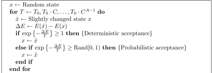
In order to find the quantized image minimizing the energyE(g) we make use ofSimulated Annealing (Algorithm 1) as described in [5]. We assume that the algorithm parameters such asβ and µgs are known in advance (more on this
later). The algorithm searches a state minimizing an energy function such as x←Random state
forT ←T0, T0·C, . . . , T0·CA−1 do ˆ
x←Slightly changed statex ∆E←E(ˆx)−E(x)
if exp−∆ET ≥1then{Deterministic acceptance} x←xˆ
else if exp−∆ET ≥Rand[0,1)then{Probabilistic acceptance} x←xˆ
end if end for
Algorithm 1: Simulated annealing
ourE(g). First, it is initialized with a random state. Then, the state is changed a little (e.g. in the case of quantization by changing the classification of a single pixel) and accepted if this change decreases the state energy. If the energy does not decrease, the state is accepted with probability equal to the Boltzmann factor [5]
e−∆E/T. (2.12)
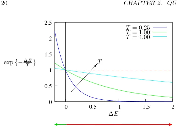
A parameterT (not to be confused with ˆT from (2.8)), called the temperature because of its foundation in physics, determines to what extent energy increases are allowed.
more deterministic more probabilistic 0
1.5 2 2.5
0 0.5 1 1.5 2 0.5
1
∆E
T= 4.00 T= 1.00 T= 0.25
exp−∆ET T
Figure 2.8: Acceptance probability at different temperatures.
The starting temperature T0 determines how randomly different states are visited. It should be high enough to allow all possible states be visited at the start of the algorithm, but if chosen too high, the algorithm needs too many steps to settle down [5]. The cooling factor C ∈ (0,1] determines the rate at which the temperature decreases. If the temperature is dropped too fast, the algorithm can get trapped in local minima.
2.3
Modified Metropolis Dynamics
To optimize Algorithm 1 for massively parallel systems we chose to use Modified Metropolis Dynamics (MMD) as given in [14]. There, the comparison with a random value from the range [0,1) is substituted with a comparison with a predetermined global threshold αin the range (0,1). This means that we can replace the exponentiation with a precalculated logarithm. Another change is that the calculation of the energy is performed local to each pixel, i.e. each pixel has its own energyEs=E(gs) which is optimized. This results in an algorithm in which all pixels can be processed in parallel.
These changes result in Algorithm 2. The energy function now becomes (C2s are the pair cliques pixelsbelongs to)
E(gs) =
ln(√2πσgs) +
(ys−µgs)
2
2σgs
2
| {z }
fidelity
+ X
(s,t)∈C2s
βδ(gs, gt)
| {z }
regularity
. (2.13)
ran-2.4. CHOOSING PARAMETERS 21
g←Random quantized image
forT ←T0, T0·C, . . . , T0·CA−1 do ˆ
g←Slightly changed quantized imageg
fors∈S do
∆Es←E(ˆgs)−E(gs)
if ∆Es≤0then{Deterministic acceptance} gs←gsˆ
else if ∆Es≤T· −lnαthen{Probabilistic acceptance} gs←gsˆ
end if end for end for
Algorithm 2: Modified Metropolis Dynamics
dom value in Algorithm 1: the comparison exp
−∆ET
≥Rand[0,1)
becomes
∆Es≤T · −lnα.
(2.14) This means that forα close to 0 all new states are accepted, while forα= 1 only energy decreases are accepted.
If the standard deviations of quantization classes within input images do not vary much, then we can simplify the energy function, assuming the standard deviations are constant. Therefore we define the following energy function:
˜
E(gs) = (ys−µgs)
2+ X (s,t)∈C2s
˜
βδ(gs, gt), (2.15)
where ˜β = (2σgs
2)β. The logarithmic terms eliminate each other in the calcu-lation of ∆Es. ˜E(gs) minimizes (2σgs
2)E(gs), which has the same minimum as E(gs) if all standard deviations are the same.
2.4
Choosing Parameters
Evolutionary Design
In this chapter we describe the Evolutionary Design methodology, used in this project for the implementation of a parallel quantization algorithm.
3.1
Current Practice
In this section we describe development methodologies for parallel systems which are currently in use at the company Oc´e and the CADTES research group at the University of Twente.
3.1.1
Oc´
e
Currently, functionality of parallel image processing systems is designed in C us-ing a common framework with multiple flavors. Each employee has the freedom to some degree to use his own methods of supporting his or her development. In the case of image processing, some people choose to model their algorithm in Matlab. When they have finished this implementation and have a working model, they implement the algorithm from scratch in Very-High-Speed Inte-grated Circuit Hardware Description Language (VHDL) or some other target language.
The benefit of using C is that it is fast, so it is often possible to approach the speeds of the hardware implementation, where full sized images can be processed within acceptable time. However, because C is sequential, it does not map well to parallel architectures, such as Field Programmable Gate Arrays (FPGAs).
The benefit of using Matlab, is that it increases development speed, because of its higher level constructs. Matlab programs are also more parallel in nature, which makes them easier to map to parallel hardware. The downside is that a Matlab implementation is not as fast as one in C and that tests therefore have to restrict themselves to downscaled versions of the problem.
Both the C and Matlab approaches lack a link between the specification of the system and the final implementation.
3.1.2
CADTES Group
At the Computer Architecture Design & Test for Embedded Systems (CADTES) group, algorithms contained in multiple parallel processes, are specified using
3.2. ALTERNATIVES 23
a mixture of Matlab and C code. The Matlab parts are then transformed into C code, after which a tool is used to separate parallel and sequential parts and map these to different parts of the hardware.
A recent development is the use of the Matlab tool Simulink to divide an algorithm into blocks of separate functionality. These blocks can each be imple-mented in a different language. Performance critical parts can be impleimple-mented in C, while less critical parts can be written in high level Matlab code. It is even possible to implement blocks using VHDL, so these parts can actually run on hardware. Using this method, different parts of the system can be described at different levels of abstraction, whatever is more convenient. This also makes it easier to test a specification against the implementation in hardware.
This methodology creates a bridge between the specification of the algorithm and the implementation and can be used to model parallel systems. However, it still makes use of sequential parts (C and to a lesser degree, Matlab).
3.2
Alternatives
This section introduces two methodologies which address some of the issues mentioned in Section 3.1.
3.2.1
Blaauw and Brooks
Blaauw and Brooks distinguish three aspects of the design of a system. • Thearchitecture defines a minimal behavioral specification of a system. • Theimplementation defines the inner workings of the system.
• Therealization defines specifics of how a system is actually built. According to Blaauw and Brooks in [4] using natural languages such as En-glish for the specification of a computer architecture is sensitive to ambiguities. To counter this, specifications can be written in a formal language, such as Z [13]. Programming languages can be used as an executable formal language for the specification of computer architectures.
Following Blaauw and Brooks, such a language should be:
High level so each desired function can be expressed directly, without having to bother with things like memory allocations and implementation of ba-sic data structures. It also avoids suggesting an implementation, which otherwise would restrict the developer.
Executable to permit demonstration to the user early in development, so the user can actively influence the functionality of the architecture. This is important, because the architecture cannot be proved or verified to be correct. It is desirable for the language to be interactive, to keep the edit-compile-run cycle short and to make it possible to easily determine the state of the system.
Established so that it is well tested and debugged and code can be shared with the community of language users.
Structured so it encourages a clear design structure with subordinate func-tions, which helps top down design.
The language Blaauw and Brooks use for their specifications is A Programming Language (APL).
Because of the use of APL, Blaauw and Brooks can develop their specifica-tion faster than they would have in C. APL being an array language, also makes it possible to model parallel algorithms.
One downside of using such a high level language is that these languages are less efficient than the target hardware language, especially when they are interpreted. This means that the problem often has to be downscaled to run the specification at a reasonable speed. Another downside of this methodology is that it does not specify how to transform the specification into an implemen-tation on the hardware.
Conceptual Integrity
One method of specifying a system is to divide the system into parts and give the responsibility for each part to a different person. When the specifications of the different parts are ready, it may well be that the specifications are incompatible, because there was no supervision on the whole system.
Blaauw and Brooks claim that it is better to have a single person be responsi-ble for the design of the entire system, which should keep the specification of the system consistent. This single person should then delegate the implementation of parts of the system to his subordinates.
The use of a language like APL assists this idea, because its concise and powerful notation can simplify specification and thus make it possible for a single person to grasp the design of larger systems.
3.2.2
Bernecky
In [3] Bernecky splits the design of an algorithm on hardware into three phases, each producing a different model, followed by a transcription phase. These phases are:
1. the concise model in which the problem and solution are researched and understood. This results in a functionally complete prototype, implement-ing the architecture.
2. theintermediate model introduces the data structures and algorithms that are to be used. This results in a prototype specifying the implementation of the system.
3. thedetailed model is a reflection of the implementation as implemented in the target language.
When the detailed model is obtained, it is translated into the target hardware language in thetranscription phase.
3.3. EVOLUTIONARY DESIGN 25
language
architectural
domain
language domain
target
Abstraction
Level
Functionality
incremental prototyping
development
transformational
Figure 3.1: Path of evolutionary design through the design space.
3.3
Evolutionary Design
Our design methodology also makes use of a high level language, just like the methods of Blaauw and Brooks, and Bernecky. Evolutionary design globally consists of two phases (Figure 3.1). During the first phase, Incremental Pro-totyping, the problem is researched until a high level, functionally complete implementation exists. After that, during the Transformational Development phase, in a series of transformation steps, the code is refactored into a form resembling the structure of the target language. The last step in this procedure is a translation from the high level language into the final implementation lan-guage. This translation can be automated by implementing a (simple) compiler. In order to be able to do these things, the high level language that is used has to have some extra qualities with respect to those given by Blaauw and Brooks. The language should additionally be:
• able to support programming on different abstraction levels. This makes it possible to apply Transformational Development.
• conceptually close to the target language (e.g. use an array language to develop for a parallel processor array). This reduces the effort needed for Transformational Development.
3.3.1
Incremental Prototyping
The goal of this phase is to learn about the various aspects of the development: functionality of the system, the target architecture and the description language. The functionality of the system is built at a high abstraction level, one function at a time. The only guidance in this phase of development are the requirements of the user, so communication with the user is important. Because we use an executable description language, we can directly show the behavior of the system, without ambiguities.
knowl-low trade−off reorganization translation
template
Abstraction Level high
Figure 3.2: Transformational development
functional prototype
reference prototype
expanded
prototype implementation final equivalent
prototype Transformational Development Time
Incremental Prototyping
Evolutionary Development
Trade−off Reorganization Template Translation
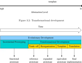
Figure 3.3: Overview of Evolutionary Design: (Sub)phases are passed through from left to right in time. The nesting of the different subphases are also shown.
edge is needed in later phases to make useful design decisions, and therefore is included here.
If the programmer is not yet comfortable with the description language, this phase presents a good opportunity to get familiar with it. The functional prototyping presents an interesting learning vehicle.
After the prototype is functionally complete, the result of this phase is a first simple, but functionally complete, implementation of the system. This method-ology also makes it possible to transform the specification of the algorithm into the final implementation on the hardware.
3.3.2
Transformational Development
Transformational development is the journey from a high to a low abstraction level. During this journey we step through a couple of design subphases (Fig-ure 3.2). Each subphase results in a specific end result. Although the main development momentum is directed top-down, there is also a small bottom-up step: the template phase.
3.3. EVOLUTIONARY DESIGN 27
Trade-Off Subphase
The goal of this subphase is to change the functional description from the In-cremental Prototyping phase into a description generating the same output as the hardware implementation. This means that all descriptions after this sub-phase have exactly the same behavior and thus can be tested by comparing their output. So, this phase is used to remove all remaining uncertainties from the description.
The activities during this phase consist of choosing specific algorithms and data types and investigate possible trade-offs, e.g. adapt bit precision to the target hardware. The influences of these activities can be measured by compar-ing the results with those of the Incremental Prototypcompar-ing phase, which acts as a ‘perfect’ reference. The extent of the influences of the trade-offs have to be determined together with the user of the system.
The main risk in this phase is making wrong decisions because of lack of knowledge of the architecture or the problem that has to be solved. This risk can be reduced by performing tech-probes during the Incremental Prototyping phase and to perform this subphase together with the future user of the system. At the end of this subphase there should be a description of the system for which the behavior is definitive: only the implementation can change. This is where the influence of the problem domain (and the system user) stops and from which the development is guided by the target architecture.
Reorganization Subphase
The goal of this subphase is to transform the system description into a form where all operations are performed in the same way as on the target hardware. If we interpret the Trade-Off Subphase as describing theWhat? of the system, the Reorganization Subphase describes the How?. Possible transformations in this subphase are changing parallel instructions as explicit loops and breaking up complex expressions.
Because in this subphase the behavior of the description is already fixed, all descriptions can be verified against each other. This makes it easy to find mistakes made during the transformation.
The result of this phase is a description of the system which mimics the final implementation both in behavior as in structure.
Template Subphase
The goal of this subphase is to transform the description of the Reorganiza-tion Subphase into a form which is easy to parse and translate into the target hardware language.
helpful if there are a lot of similar constructs that can be abstracted into one code template.
Code templates are the link between the system description and the target hardware language. Therefore, the templates are a perfect location to check for additional requirements of the hardware, such as calling conventions.
The result of this phase is a system description which can be translated into the target hardware language by a simple translator. This translator has to do little more than expanding code templates into the target hardware instructions.
Translation Subphase
The goal of this subphase is to translate the system description from the Tem-plate Subphase directly into the target hardware language. This can be done automatically by using a (simple) compiler, which is written together with the code templates.
There are two possible sources of errors in this subphase: the parser imple-mentation of the translator and the impleimple-mentation of code templates into the target hardware language. The possibility of a faulty parser can be reduced by using a specialized tool for writing compilers and translators. A typing error in a code template can often be corrected, but if the error is caused by wrong assumptions about the hardware it may be needed to fall back to the Template Subphase or an even earlier phase.
The result of this phase is a working implementation of the described system with identical behavior as established at the end of the Trade-Off Subphase.
3.4
Intended Benefits
Here we give some of the possible benefits of Evolutionary Design.
3.4.1
Higher Productivity
Our main objective with Evolutionary Design is to make development easier and more productive. The use of an executable language gives early feedback during development, which makes development more dynamic. This makes it easier for users to make sure that they get the product they want and helps developers to verify and debug their implementations.
Using Transformational Development, we make sure that each development step is consistent and correct with respect to the previous, higher level state of the design.
3.4.2
Error Recovery
3.4. INTENDED BENEFITS 29
Algorithm 1
Architecture 1
Algorithm 2 Common Code Templates
Algorithm 3
Architecture 2
Figure 3.4: Increasing portability by using common code templates. Algorithms are implemented in terms of these code templates. For each code template there is an implementation on each architecture.
3.4.3
Portability
The Template subphase can be used to identify common abstractions between different hardware implementations. This way, common code templates can be developed for different architectures. When this is achieved, development can focus on implementing towards these templates (of which there are few) instead of towards each separate piece of hardware. This way, existing algorithms can be implemented on new hardware after an implementation for the common code templates has been developed for it. Conversely, new algorithms written in terms of the common code templates can run on all machines supporting these templates (see Figure 3.4).
3.4.4
Domain Expert Programming
One of the possible benefits of Evolutionary Design is that all domain spe-cific problems are solved in the Incremental Programming phase. If the higher level language is simple enough to be understood by domain experts, they can perform the Incremental Prototyping phase themselves. When the Incremen-tal Prototyping phase is over, system engineers can take over and start at the Trade-Off subphase, with feedback from the domain experts.
Linedancer
In this chapter we introduce the hardware architecture used in our research: the Linedancer, which is manufactured by Aspex, a UK based fabless semiconduc-tor company specializing in high performance, software programmable, parallel processors based on associative technology. We give a short introduction on par-allel architectures, followed by the specific properties of the Linedancer itself. The chapter concludes with performance measures of some of the instructions of the hardware.
4.1
Parallel Architectures
In this section we give a short introduction into parallel architectures.
4.1.1
Processor Architecture Taxonomy
In 1966 Flynn divided processor architectures in terms of their data and instruc-tion multiplicity. This has lead to Flynn’s Taxonomy of four different types of computer architectures (see Table 4.1.1).
The Single Instruction Single Data (SISD) architecture is the one typically found in modern day PCs: each instruction acts on a single data unit.
The Single Instruction Multiple Data (SIMD) architecture has also made its entrance into consumer computers when Intel introduced their MMX Pentium models, later followed by AMD’s 3DNow!. These technologies provide instruc-tions, which enables one to apply a certain instruction to multiple data units at once. E.g. vector additions could be performed using only one instruction, instead of doing the addition for each vector element explicitly.
The Multiple Instruction Single Data (MISD) is more or less a theoretical architecture because its use has been very limited. Some would place systolic
Instructions Single Multiple
Data Single SISD MISD
Multiple SIMD MIMD
Table 4.1: Processor Architecture Taxonomy according to Flynn.
4.1. PARALLEL ARCHITECTURES 31
arrays into this category.
The Multiple Instruction Multiple Data (MIMD) architecture has been around for a long time. Examples can be found in specialized high performance parallel computers such as developed by the Cray1 supercomputer company. During the last decennium MIMD also made its entrance into the PC world as multi processor systems became more commonplace. Another example of MIMD are rendering farms, which are used for rendering of computer animations and sim-ulations. These consist of tens to hundreds of PCs and communicate through a high speed network. Finally, the trend of distributing the execution of brute force algorithms via the Internet can be seen as a form of MIMD. In this scheme, private persons are asked to donate the idle time of their computers to help in some calculation. Examples of this kind of MIMD are the SETI 2 [2] and RC5–723 [1] projects.
4.1.2
Benefits of Parallel Architectures
At first glance the use of parallel architectures only has benefits. If more pro-cessors work at a certain task, then the task is completed sooner than when only one processor is used.
While this is true (you could always use only one processor and finish the work in the same time) the benefit is not linear: doubling the number of pro-cessors generally does not half the processing time.
To understand this, we define the term speedup. If Tseq is the time taken by the most efficient sequential algorithm to perform a task andTpar(n) is the time taken by the most efficient parallel algorithm to perform the same task when running onnprocessors, then the speedupSn is the ratio between these times, i.e.Sn=Tseq/Tpar(n). So, if a parallel algorithm running on 8 processors performs a task twice as fast as a sequential algorithm then the speedup is 2.
In practice, most parallel algorithms also have a sequential component, e.g. for managing the communication between the processors. If we call the fraction of sequential operations in an algorithmf, then we can deriveAmdahl’s law:
Sn≤ f+ (11
−f)/n. (4.1)
When we take the limitn→ ∞we see that this reduces toSn≤ 1
f. So, if our algorithm consists for 5 percent of sequential algorithm we can hope to achieve a speedup of 20 or less. This tells us that just adding more processors does not help us much and that we will have to carefully evaluate the added value of multiprocessing for each problem.
Note, however, that the most efficient sequential algorithm does not have to have the same model as the most efficient parallel algorithm. So, when developing an algorithm, care should be taken not to simply try and implement a known sequential algorithm on a parallel architecture. The most efficient parallel algorithm could be completely different. Amdahl’s law should therefore be kept in mind, but it should not discourage the developer in finding new and more efficient models for his problems.
1
http://www.cray.com
2
a project to find extraterrestrial intelligence by analyzing data from radio telescopes.
3
PE
PE PE PE PE
(a)
PE PE PE
(b)
Figure 4.1: Expanding a mesh (a) requires more PEs than expanding a string (b).
4.2
Hardware Architecture
The Aspex Linedancer parallel processor array is a member of the SIMD family of processor architectures. The Linedancer is used for image processing tasks, e.g. color correction [6]. Our current system, the Linedancer development board, is mounted on a PCI card and contains 2 Linedancer chips. Both of these chips contain an array of 4096 PEs, each with its own memory of almost 200 bits. Control of the array is maintained by the processor of the machine the Linedancer is installed in and an onboard RISC processor. These are referred to as the System Control Computer (SCC) and the Instruction and Data Stream Manager (IDSM) respectively.
4.2.1
Scalability
While in most SIMD architectures the PEs are arranged in meshes, the PEs in the Linedancer are arranged in a string (Figure 4.1). So, in order to increase the number of PEs, multiple Linedancers can be connected serially, while a mesh would require adding a lot more PEs to maintain its structure. This improves the scalability of the array and reduces the complexity of the chip’s design. However, it also increases the communication time between PEs, because there are less communication channels.
4.2.2
Memory Transfers
Memory transfers from, to and inside the Linedancer can be divided over a memory hierarchy, consisting of Tertiary Data Store (TDS), Secondary Data Store (SDS), Primary Data Store (PDS) and the PE memory (Figure 4.2). TDS is the main memory of the system that contains the Linedancer (e.g. a PC). Typically this memory is only used to store the input and output of the entire program.
4.2. HARDWARE ARCHITECTURE 33
Linedancer PC Linedancer
TDS SDS PDS PE memory
PE #1 PE #2 PE #3
PE #4096
SDS PDS PE memory
PE #1 PE #2 PE #3
PE #4096
For each PE there is a 64 bits PDS memory. This acts as a buffer between the SDS memory and the PE’s data registers, enabling streaming by double buffering. Transfer between SDS and PDS is controlled by the Secondary Data Movement Controller (SDMC): a DMA controller that can be programmed to do all kinds of transfers and divides the SDS data between the PEs, one item at the time. E.g. the SDMC makes it possible to process an image either row-or column-wise row-or replicate data across multiple PEs.
4.2.3
Associativity
PE memory is divided in two parts, Extended Memory (EXT) and Content Addressable Memory (CAM). The CAM part can be addressed based on its contents instead of its physical address. Because of this, searching data in the PEs is very easy. It also makes the addressing independent of the array’s string size, so your code does not have to be altered when the number of Linedancers is expanded for increased performance.
The associative memory relies on the use of a number of tag registers and one activation register for each PE. The tag register of a PE can be set based on the contents of its CAM using theTaginstruction. This is illustrated by an example.
In Figure 4.3(a) the tag register (T) is set for PE with a specific part of their memory (M) set to 010. The activation register determines which PEs can be written to. TheActivate instruction can set the activation register on all PEs or based on one of the tag registers. In Figure 4.3(b) the activation register (A) is set for for those PEs which did not match the pattern 010, i.e. those which do not have their tag register set and in Figure 4.3(c) the pattern 10 is written to the activated PEs.
4.2.4
Communication
Data inside the registers can be freely moved between the PEs. The number of cycles this takes depends on the distance between the PEs involved.
The IDSM can directly write scalar data to activated PEs. This is done by
theWriteinstruction.
It is possible to transfer the contents of the tag registers through the array, one PE at the time. This can be used to access PEs based on the contents of their neighbors.
4.2.5
Segmentation
By default the array behaves as a string with its extreme ends connected. The PEs can be split up into multiple segments. These segments each operate in-dependently as if they were physically distinct Linedancers, without the pos-sibility of communication between them. This way, multiple Linedancers can be emulated on a single physical device. Segments are defined by theSegment
4.2. HARDWARE ARCHITECTURE 35
0
0 0 0 0
0
0 0
0 0 0
0 0
0 0 0 1
1
1
1 1 1 1 1 1 1 1 1 1 0 1 0
M T A 1 1 0 0 1 1 0
(a) The tag register (T) is set for matching PEs.
0
0 0 0 0
0
0 0
0 0 0
0 0
0 0 0 1
1
1
1 1 1 1 1 1 1 1 1 0 1 0 1 M T A 1 1 1 0 0 1 1 0
(b) The activation register (A) is set for PEs where tag register (T) is not set.
0 0 0 0 0 0 0 0 0 0 0 1 1 1
1 1 1 1 1 0 1 0 1 M T 1 0 0 0 1 1 1 0 1 0 1 A 1 1 0 0 1 1 0 0 0
(c) Data is written to PEs with set activation registers.
Instruction Description RTS(Add) Addition RTS(Sub) Subtraction
RTS(AddSub) Either addition or subtraction, depending on a special bit
RTS(Assign) Assignment, within a single PE or from one PE to an-other
RTS(le) Less than of equal comparison RTS(Xor) Bitwise Xor
Table 4.2: Some of the RTS instructions that can be used on the Linedancer.
4.2.6
Arithmetical and Logical Operations
The only arithmetical operations that a PE can perform on the data inside its memory are addition, And, Orand Xor. These can all be performed innormal and complement mode. When in complement mode, one of the operands is complemented before the operation. Non-basic operations, such as division and subtraction are implemented in terms of the four basic operations. Because the ALU is only 2 bits wide, calculations per PE are generally slower than those done by a PC because they have to be emulated and performed serially. This emulation is done by so called RTS macros Table 4.2. An advantage is that PE memory can be accessed on bit level: i.e. it is possible to access and operate on 3–bit quantities inside the memory.
4.3
Programmer’s Interface
The programmer’s interface consists of the software tools used to compile a program and a number of supporting libraries.
4.3.1
Software Tools
The programming language is C, extended with aop blocks, which contain Linedancer instructions. If the SCC and IDSM are different processors, compil-ing results in two separate binaries; one for each processor. The SCC program is the main entry point: it initializes the Linedancer and starts the separate IDSM processors.
4.3.2
Threads of Execution
4.4. PERFORMANCE 37
Instruction Cycles
Tag 4
Segmentation 2
Write 2
Activate 2
Table 4.3: Linedancer operations running with a constant number of cycles.
4.3.3
Libraries
Aspex has written some higher level libraries on top of the basic Linedancer instructions, which can make programming the Linedancer a bit simpler.
Image Library
This library takes care of splitting image data loaded in the SDS into tiles of smaller image parts. These tiles can then be uploaded to and from the PDS. It also takes care of configuring the SDMC parameters, which can be difficult to understand.
Message Queue Library
This library makes it possible to create different message queues between pro-cessors. This can be used to transfer configuration information (e.g. from the command line) between the SCC and the IDSM or to return status information from the IDSM to the SCC. Because the queue transfer operations can be made to block they are also an excellent tool to synchronize the different threads.
4.4
Performance
Here we present the results from testing the performance of some of the Linedancer operations that we used.
4.4.1
Constant Time Instructions
The instructions used for associative operations take constant time (Table 4.3. However, multiple occurrences of these instructions can be optimized into one occurrence.
4.4.2
Linear Time Instructions
Basic arithmetic and logical operations depend linearly on the bit widths of their operands. After some tests we were able to calculate the exact dependency (Table 4.4, w is the width of the result and operands). For most operations with a cycle count dependent on the bit widths of the operands, the number of cycles is smaller if the operand width is even than when it is odd. This is because of the 2-bits ALU, which is only used if the operand widths are even.
4
Instruction Cycles
Even Width Odd Width pdTransfer4 14 + 12w 14 + 12w
RTS(Add) 2 +w 2 + 2w
RTS(Sub) 2 +w 2 + 2w
RTS(AddSub) 2 + 2w 2 + 4w
RTS(Assign) (local) 2 +w 2 + 2w
RTS(le) 6 +w 8 + 2w
RTS(Xor) 4 +w 4 + 2w
Table 4.4: Linedancer operations which are linearly dependent on the bit width.
Because the test setup for the pdTransfer instruction demanded that both a Load and a Dump were done, we only have results from both calls together. The number of cycles taken by only one of these calls is probably one half of the number in Table 4.4, but this has not been verified.
4.4.3
Slow Instructions
In Figure 4.4 the relation between bit width and the running time in cycles is shown for the RTSMult and RTS(Div) instructions. These instructions are slow: the multiplication of two eight bits numbers takes 114 cycles, while the addition of those numbers only takes 10 cycles. RTS(Mult) and RTS(Div) also have worse than linear behavior with respect to the number of bits. RTS(Div) is dependent on whether it is applied to integers (Int) or cardinals (Card). Based on these measurements, RTS(Mult) and RTS(Div) should therefore be avoided whenever possible.
4.4. PERFORMANCE 39
0 100 200 300 400 500 600
0 2 4 6 8 10 12 14 16
Cycles
Operand Width
RTS(Mult) Even RTS(Mult) Odd
(a) RTS(Mult)
0 200 400 600 800 1000 1200 1400
0 2 4 6 8 10 12 14 16
Cycles
Operand Width
RTS(Div) Int Odd RTS(Div) Int Even RTS(Div) Card
(b) RTS(Div)
Figure 4.4: Dependency of the number of cycles on the operand width for the RTS(Mult) and RTS(Div) instructions.
0 2000 4000 6000 8000 10000 12000 14000 16000 18000
0 20 40 60 80 100 120 140
Cycles
Distance (# PEs) RTS(Assign) Remote
Implementation
In this chapter we introduce the decisions we made while implementing the quantization algorithm from Chapter 2 on the Linedancer (Chapter 4). This implementation is supported by the Evolutionary Design methodology intro-duced in Chapter 3.
When the algorithm is run, the parameters are first chosen to likely corre-spond with the actual data. Next the quantized image is found by minimizing the energy function using Simulated Annealing.
Our methodology applied on the Linedancer has only been used to write the parallel part of the implementation, the ISM thread. This was done, because this is the most difficult part of the hardware to program, comparable with assembler code. Also, the code for the other threads is very similar for different problems, so these are a lot less sensitive to change than the ISM thread.
5.1
Preparation
We chose the J programming language [8] as the high level language to apply our methodology with. For this we had three reasons:
1. it was already used in my working environment;
2. it was a totally different programming language than that I had been used to using, so I was interested in its use;
3. it fulfilled the requirements mentioned in Chapter 3.
J was developed as a derivative of the APL programming language, which was popularized by Kenneth Iverson, first as a mathematical notation, later as a programming language while at IBM.
J has powerful primitives and has a very mathematical inclination, which helps when specifying complex algorithms. J is a language with arrays as pri-mary data type, which results in a parallel approach of the manipulation of data. Allocation and deallocation happen automatically and all data accesses are by value, so there is no use of pointers. These qualities make J easier to use and less error prone than languages such as C. Compared to e.g. Matlab, J is very concise in notation and is very light weight: the installation is only 20
5.2. INCREMENTAL PROTOTYPING 41
MB. Functions are first citizens in the J language, but it is not a strict func-tional language, such as Haskell or Miranda, because it allows for side effects, has variables and control flow constructs such asIf,For, etc.
The makers of J have optimized it quite a bit; e.g. some combinations of keywords are recognized and have an optimized implementation.
This chapter contains snippets of J code to give a general idea of what kind of transformations are done. It does not matter if the code is not entirely understood. In Appendix A you can find a short introduction to J, which should help understand the J code used here.
5.2
Incremental Prototyping
Before the implementation of the quantization algorithm we tried different im-plementations of Simulated Annealing programs found in literature to learn about the theory behind it. Because I wrote these test programs in J, this was also a way to get familiar with the programming language. During my intern-ship I had already worked with the Linedancer, so I had a general idea how the hardware architecture behaves.
The first implementation in J can be found in Section B.1.1. The annealing procedure is located in the lines 1–22. This implementation serves as the root of our development efforts.
5.3
Transformational Development
We now give an overview of how the different subphases of Transformational Development were passed through during the implementation of the quantiza-tion algorithm. This is done using concrete examples from the implementaquantiza-tions in J. For an introduction to J primitives, we refer to [9]. Comments in J start withNB..
5.3.1
Trade-Off Subphase
The goal of this subphase is to change the functional description from the Incre-mental Prototyping phase into a description generating the same output as the hardware implementation. We quantized some test images using the program Irfanview and used these results as a reference. We chose a threshold of 5% misqualified pixels to represent a ‘good enough’ quantization. This was used to compare different trade-offs in this subphase.
Tiling
Our implementation uses one PE for each pixel in the input image, because this is the massively parallel part of the algorithm. The number of PEs in the Linedancer is limited (although it can be expanded), so the number of pixels that can be processed together is also limited.
Figure 5.1: Tiling: the input image is cut into blocks fitting inside the Linedancer and processed in sequence by the Simulated Annealing algorithm.
• It is a simple method, so it would not complicate the algorithm any further. • Some tests on an early J model gave the impression that non overlapping
tiling would not have a large influence on the algorithm.
We chose to minimize the number of SDMC transfers, and not communicate between tiles in order to maximize the number of parallel calculations within a tile. This was done to maximize calculations, which the Linedancer is good at, and minimize communication overhead.
Note that this way of tiling increases the locality of the algorithm, because there is no influence between data in different tiles.
Round Off
Although hinted on in the documentation, the Linedancer does not support floating point numbers in the PEs. This was confirmed by someone from Aspex. Therefore, we would have to round off values or use fixed point arithmetic if more than integer precision would be needed.
The only parameters that are candidates for round off are: ˜
β the inverse of the Simulated Annealing temperature, which can be interpreted as the weighting factor between fidelity and regularity; µgs the mean values for each quantization class;
−T·lnα the threshold in the Simulated Annealing algorithm.
We tested the range of useful ˜β values for our test set of images. We chose a set of possible ˜β values and determined the value for which misclassification was minimal for each image. This gave us a collection of ˜β values, which we assumed as the range needed for our algorithm. This range lay between 20 and 88 and it was found that integer values are sufficient and that the use of fixed point math is unnecessary. 7 Bits are sufficient to represent each integer value within this range.
We tested the effects of using integer values for µgs. The misclassification
5.3. TRANSFORMATIONAL DEVELOPMENT 43
1
0
0
1
0
1
0
1
W = 10
XOR
1 2 3 4 5 6 7 8 9 10
1
1
0
(a) First step: calculate the Xor of the taps from the current state.
right shift
0
0
1
0
0
1
1
0
1
1
W = 10
1
4 8 9 10
3
2 5 6
1 7
(b) Second step: shift to the right to get the new state.
Figure 5.2: A 10 bits wide Linear Feedback Shift Register. A 0 is shifted out and 1 Xor 0 = 1 is shifted in.
We tried to find a suitable rounding for −T ·lnα but we could not find any. Even replacing this value with 0 had no effect. This essentially means that transforming the algorithm into a deterministic one (one which only lowers the energy) did not influence the outcome. However, in order to not over-simplify the algorithm used to evaluate the methodology, we rounded off threshold values to integers instead of replacing them with 0.
Random Number Generator
We chose to use a Linear Feedback Shift Register (LFSR) to generate pseudo random numbers on the Linedancer. Figure 5.2 shows the schematic of a LFSR. A LFSR is a rotating shift register, with a bit width ofW. Its state is initialized with a non-zero value, the seed. Pseudo-random numbers are generated by calculating a new state, which depends on the values at some of the bit positions: thetaps. The calculation of a state involves Xor-ing the bits at the tap locations and inserting the result at the least significant bit position, shifting the other bits one position to the right.
Some combinations of bit widths and tap positions give a sequence of states covering all possible states, except zero: these combinations are calledmaximal. Maximality is a desirable property for the random number generator, because it maximizes the period of possible generated numbers. More on Linear Feedback Shift Registers can be found at [16].
the LFSR is maximal, all states except zero are possible, but if it is seeded with zero, it stays zero. When we haveN different states, states lie within a range of{0, N−1}. This means that the values obtained from the LFSR have to be transformed into the range of the states.
Our first attempt at this, was by decreasing the value of the LFSR with 1 and use the remainder after division byN. This can be found in Section B.1.2 in lines 13–19 from which the following lines have been taken, with some comments added for clarification (y.is the input image,randomis a function implementing a LFSR):
NB. Initialize seed to random values. seed=. ? ($ y.) $ (# , y.)
NB. Calculate new seed using a LFSR of 10 bits wide and taps at NB. bits 10 and 7.
seed=. (10 ; 10 7) random seed
NB. Map seed to state by subtracting one and calculate the NB. modulus with the number of labels LABELS.
nstate=. LABELS | <: seed
This approach was wrong. First of all it uses the number of elements in the image to determine the maximum seed value, for which there is no good reason. Second, it still allows for seeds being initialized to 0. This error was only found and corrected in a later subphase, which is discussed later.
We tried to find a suitable bit width for the random number generator. We compared the output of our model using the LFSR implementation with a version using the built in J version by looking at the images. This made us decide on a bit width of 12 for the LFSR.
5.3.2
Reorganization Subphase
The goal of this subphase is to transform the system description into a form where all operations are performed in the same way as on the target hardware.
Simulation Length
Because we calculate everything in the same way and with the same precision as we will do on the Linedancer, we can reduce the number of iterations of the algorithm during tests. This reduces the time needed to verify the correctness of a translation step.
Globalization
All functionality is gathered within a single function and all variables represent-ing memory fields are made global. This is done to mirror the situation on the Linedancer, where all memory fields are also essentially shared. This may look as bad programming practice, but actually this is the introduction of a lower implementation level.
Resource Assignment
5.3. TRANSFORMATIONAL DEVELOPMENT 45
variables to memory fields. Therefore, we used an Excel sheet for ‘keeping score’: keeping track of which bits of PE memory were used for which variable in the J model and warning us when we used too much space. When going through the Reorganization subphase, we bring our model code closer to the assignments used in the Excel sheet. We rename variables so their names include the offset and size they will have in PE memory. A variable nameDUMMYis changed to
DUMMY 4 16meaning that it is a 16 bit wide value, located at bit offset 4.
Resource Sharing
During the reorganization subphase, the code is getting more and more dis-connected with the original algorithm and becomes a sequence of very simple instructions. Sometimes this actually helps in simplifying the code. For exam-ple the variablemuin Section B.1.4, lines 19–49 can be merged with the use of the variablea. The result of this operation can be seen in Section B.1.5, lines 23–53. Because variables correspond to memory fields during the translation, this simplification frees up some extra bits in each PE for other uses.
Expansion
We expand parallel constructs that will have to be done in loops on the Linedancer. One example is the expansion of the code which calculates the energy of a state. In Section B.1.2 the following code can be found in line 21:
NB. Calculate the likelihood part of the energy by squaring the NB. differences of the pixel values and label means.
lhood=. *: y. - state { MU
![Figure 2.1: Typical office scan: text and charts.[Typical office scan]](https://thumb-us.123doks.com/thumbv2/123dok_us/1162546.1146371/14.595.221.320.550.689/figure-typical-oce-scan-text-charts-typical-oce.webp)