Copyright1999 by the Genetics Society of America
Multiple Interval Mapping for Quantitative Trait Loci
Chen-Hung Kao,* Zhao-Bang Zeng
†and Robert D. Teasdale
‡*Institute of Statistical Science, Academia Sinica, Taipei 11529, Taiwan, Republic of China,†Program in Statistical Genetics, Department of Statistics, North Carolina State University, Raleigh, North Carolina 27695-8203 and
‡ForBio Research Pty Ltd., Toowong, Queensland 4066, Australia
Manuscript received December 5, 1997 Accepted for publication March 24, 1999
ABSTRACT
A new statistical method for mapping quantitative trait loci (QTL), called multiple interval mapping (MIM), is presented. It uses multiple marker intervals simultaneously to fit multiple putative QTL directly in the model for mapping QTL. The MIM model is based on Cockerham’s model for interpreting genetic parameters and the method of maximum likelihood for estimating genetic parameters. With the MIM approach, the precision and power of QTL mapping could be improved. Also, epistasis between QTL, genotypic values of individuals, and heritabilities of quantitative traits can be readily estimated and analyzed. Using the MIM model, a stepwise selection procedure with likelihood ratio test statistic as a criterion is proposed to identify QTL. This MIM method was applied to a mapping data set of radiata pine on three traits: brown cone number, tree diameter, and branch quality scores. Based on the MIM result, seven, six, and five QTL were detected for the three traits, respectively. The detected QTL individually contributed fromz1 to 27% of the total genetic variation. Significant epistasis between four pairs of QTL in two traits was detected, and the four pairs of QTL contributedz10.38 and 14.14% of the total genetic variation. The asymptotic variances of QTL positions and effects were also provided to construct the confidence intervals. The estimated heritabilities were 0.5606, 0.5226, and 0.3630 for the three traits, respectively. With the estimated QTL effects and positions, the best strategy of marker-assisted selection for trait improvement for a specific purpose and requirement can be explored. The MIM FORTRAN program is available on the worldwide web (http://www.stat.sinica.edu.tw/zchkao/).
T
HE basic principle of using genetic markers to study genetic marker map throughout the genome, IM canquantitative trait loci (QTL) is well established (Sax be performed at any position covered by markers to
1923;Thoday1960;Jayakar1970;LanderandBot- produce a continuous LRT statistical profile along
chro-stein1989;Carbonellet al. 1992;HaleyandKnott mosomes. The position with the significantly largest
1992;Jansen1993;Zeng1993, 1994).Sax(1923) first LRT statistic in a chromosome region is an estimate of
used pattern and pigment markers in beans to analyze QTL position. It has been shown that IM has more
genes affecting seed size by investigating the segrega- power and requires fewer progeny than the methods
tion ratio of F2 progeny of different crosses. Thoday for direct analysis of markers (Lander andBotstein
(1960) proposed the idea of using two markers to 1989;HaleyandKnott1992;Zeng1994).Haleyand
bracket a region for detecting QTL. The basic idea of Knott(1992) proposed a regression version of interval
Sax and Thoday for detecting the association of a QTL mapping to approximate IM. Although Haley and
with a marker rests on the comparisons of trait means Knott’s method could save time in computation and
of different marker (chromosomal segment) classes. produce similar results to those obtained by IM, the
These methods, such as t -test and simple and multiple estimate of the residual variance is biased, and the power
regressions, directly analyze markers. of QTL detection can be affected (Xu1995).
In recent years, the advent of fine-scale molecular The approach of IM considers one QTL at a time in
genetic marker maps for various organisms by molecular the model for QTL mapping. Therefore, IM can bias
biology techniques has greatly facilitated the systematic
identification and estimation of QTL when multiple
mapping and analysis of individual QTL.Landerand
QTL are located in the same linkage group (Lander
Botstein(1989) proposed a much-improved method,
and Botstein 1989; Haley and Knott 1992; Zeng
named interval mapping (IM), for mapping QTL. They
1994). To deal with multiple QTL problems, Jansen
used one marker interval at a time to construct a putative
(1993) andZeng(1993, 1994) independently proposed
QTL for testing by performing a likelihood ratio test
the idea of combining IM with multiple regression (LRT) at every position in the interval. With a fine-scale
analysis in mapping. Zeng named this combination “composite interval mapping” (CIM). The approach of CIM is that, when testing for the putative QTL in an Corresponding author: Chen-Hung Kao, Institute of Statistical Science,
interval, one uses other markers as covariates to control
Academia Sinica, Taipei 11529, Taiwan, Republic of China.
E-mail: [email protected] for other QTL and to reduce the residual variance such
1204 C-H. Kao, Z-B. Zeng and R. D. Teasdale
that the test can be improved. The model of CIM in- up to digenic epistasis is considered, the relation
be-tween the genotypic value of individual i, Gi, and the
cludes one QTL and markers.Hoescheleand
Vanran-den(1993a,b),Satagopanet al. (1996), andSillanpaa genetic parameters can be expressed in the equation
andArjas(1998) used a Bayesian approach in
estima-Gi5 m 1
o
mj51
ajxij1
o
mj,k
wjk(xijxik), i51, · · ·, 2m, (1)
tion and to identify QTL. Doerge and Churchill
(1996) used permutation tests for QTL detection.
Map-ping for QTL controlling binary trait and ordinal cate- where xij is coded as1⁄2or 21⁄2if the genotype of Qj is
gorical traits is presented by Hackett and Weller QjQjor Qjqj, respectively, ajis the corresponding main
(1995) and Xu and Atchley(1996). In human and effect of Qj, and wjk is the epistatic effect between Qj
animal genetics, the mixed model, including random and Qk. The main advantage of Cockerham’s model is
effect, has been applied to QTL mapping (Xu and that it possesses an orthogonal property in modeling
Atchley1995;Grignolaet al. 1996a,b). genetic parameters.
Ideally, we would extend the current QTL mapping To assist with explaining the estimation of the genetic
models to a multiple QTL model for mapping multiple effects in the MIM model (Equation 3), the genetic
QTL in a way that QTL can be directly controlled in model in Equation 1 is expressed in matrix notation as
the model to further improve QTL mapping. In this Equation 2 (Scheme 1). In Equation 2, the column
article, a new QTL mapping method named multiple vector G contains the genotypic values of the 2mpossible
interval mapping (MIM) was developed. MIM uses mul- genotypes. The subscripts of G (1 or 0) denote the
tiple marker intervals simultaneously to construct multi- homozygote or heterozygote of the QTL in the order
ple putative QTL in the model for QTL mapping. There- of the first, second, third, · · ·, and mth QTL,
respec-fore, when compared with the current methods such as tively. The first m columns in the genetic design matrix
IM and CIM, MIM tends to be more powerful and pre- Dare the coefficients associated with the main effects
cise in detecting QTL as shown by the example in this of the m QTL, and the last m(m21)/2 columns
repre-article. In addition, MIM can readily search for and sent the coefficients of the epistatic effects among them.
analyze epistatic QTL and estimate the individual geno- Vector E contains the QTL main and epistatic effects.
typic value and the heritabilities of quantitative traits. If there is no epistasis between some QTL, some of
On the basis of the MIM result, genetic variance com- the columns for epistasis should be dropped out from
ponents contributed by individual QTL were also es- matrix D. If higher-order epistasis is considered, the
timated, and marker-assisted selection can be per- dimension of matrix D is easy to expand accordingly.
formed. The matrix D plays an important role in estimation of
genetic parameters in the MIM model.
GENETIC MODEL
Consider m QTL, Q1, Q2, · · ·, and Qm, in a backcross
STATISTICAL MODEL OF MIM
population in which there are two genotypes, QjQjand
Multiple interval mapping: Assume m QTL, Q1, Q2,
Qjqj, each with one-half frequency for a QTL, say Qj. For
· · ·, and Qm, located at positions p1, p2, · · ·, pm in
m QTL, there are 2mpossible different QTL genotypes in
m different marker intervals, I1, I2, · · ·, Im, along the
the population. Cockerham’s genetic model (C-H. Kao
genome, control a quantitative trait y. Among the m andZ-B. Zeng, unpublished results) is used to define
QTL, some may show epistasis and some may not. The the genetic parameters and model the relation between
the genotypic value and the genetic parameters. If only quantitative trait value for an individual, i, can be related
to the m putative QTL by the model flanking marker genotypes, can be found in Table 1 of
Kao andZeng (1997). To infer the joint conditional
yi5 m 1
o
mj51
ajx*ij1
o
mj?k
djk(wjkx*ijx*ik)1εi, (3) probability of the genotype of the m putative QTL, we
use the property that if there is no crossing-over
interfer-where m is the mean, x*
ij is the coded variable for the ence, the conditional distributions of the individual
pu-genotype of Qj, aj and wjkhave the same definitions as tative QTL genotypes, given the flanking marker
geno-those in the genetic model in Equation 1,djkis an indica- types, are independent. That is,
tor variable for epistasis between Qj and Qk, and εi is
assumed to follow N(0,s2). Indicator variabled
jktakes prob(Q1, Q2, · · ·,Qm| I1, I2, · · ·, Im)5
p
mi51
prob(Qi|Ii).
value one if Qj and Qk interact; otherwise its value is
zero. In this model, the first summation is for the main The joint conditional probability of the m QTL is the
effects of the m QTL, the second summation is for their product of the marginal conditional probabilities of
possible epistasis, andεiis the environmental deviation. individual QTL. We refer to pij, j51, 2, · · ·, 2m, as the
This is termed the MIM model because multiple (m) conditional probabilities of 2mpossible QTL genotypes
marker intervals are simultaneously used to construct (note that p
j’s denote QTL positions and pij’s denote
multiple (m) putative QTL in the model for QTL map- the conditional probabilities). If multiple putative QTL
ping. If QTL genotypes are known, the model tells that within a single marker interval are considered, the
indi-the quantitative trait value is indi-the sum of indi-the QTL main vidual and joint conditional probabilities of QTL
geno-effects, their possible epistatic geno-effects, and environmen- types can be also inferred directly or by a Markov chain
tal deviation, and the MIM model is a regression model. procedure (JiangandZeng1997) assuming no
interfer-However, the putative QTL genotypes denoted by x*
ij’s ence.
are usually not observed because QTL could be located Given a sample with size n, the likelihood function
in the intervals. Given observed flanking marker geno- of the MIM model foru 5(p1, p2, · · ·, pm, a1, · · ·, am,
types, the conditional distributions of QTL genotypes, · · ·, wjk, · · ·,s2) is
x*
ij’s, for QTL at specific positions, pj’s, can be inferred
based on Haldane’s mapping function (Haldane1919) L(u|Y, X)5
p
ni51
3
o
2mj51 pijφ(
yi 2 mij
s )
4
, (4)assuming no crossover interference (Table 1 in Kao
andZeng1997), and the MIM model is then a normal
whereφ(·) is a standard normal probability density
func-mixture model. For each Qj, its conditional probabilities
tion,mij’s correspond to the genotypic values of the 2m
are extracted to form a matrix Qj(note that Q denotes
different QTL genotypes in Equation 1, and pij’s
con-QTL and Q denotes the conditional probability matrix;
taining information on QTL positions are the
corre-seeKao andZeng1997). The conditional probability
sponding joint conditional probabilities. Statistically, matrices, Qj’s, j51, 2, · · ·, m, play an important role
this is a normal mixture model. The density of each in estimation of the QTL positions in the intervals.
individual is a mixture of 2mpossible normal densities
The MIM model is a multiple QTL model and its
with different meansmij’s and mixing proportions pij’s.
likelihood is a finite normal mixture. There are two
To obtain the MLEs and the asymptotic variance-covari-problems that need to be solved for the MIM model.
ance matrix of the model, the general formulas ofKao
The first is that of parameter estimation of the finite
andZeng(1997), based on the expectation and
maximi-normal mixture model. As m becomes large, the
deriva-zation (EM) algorithm (Dempsteret al. 1977), are used
tion of the maximum-likelihood estimates (MLEs) of
for parameter estimation. the QTL effects and positions in estimation quickly
be-comes unwieldy. To handle the estimation problem, the
general formulas derived byKaoandZeng(1997) are
PARAMETER ESTIMATION
used to obtain the MLEs in parameter estimation.
The second problem is how to find QTL to fit into The likelihood of the MIM model is a finite normal
the MIM model. To select QTL for the MIM model, mixture. In parameter estimation, the finite normal
a stepwise model selection procedure is proposed in mixture model can be treated as an incomplete-data
prob-strategy of qtl mapping. lem (Little and Rubin 1987) by regarding the trait and markers as observed data and the QTL as missing
data. The EM algorithm can be used for obtaining the LIKELIHOOD OF THE MIM MODEL
MLEs of the genetic parameters, and Louis’s (1982)
method can be implemented to obtain the variance-In the MIM model, the genotype of each putative
covariance matrix. QTL, Qjin interval Ij, is not observed, but its distribution
In the MIM model, when only one putative QTL (m5
can be inferred from the flanking markers of Ij based
1) is considered in a backcross population, the likeli-on the recombinatilikeli-on frequency between them. For
hood is a mixture of two normals (like IM and CIM), and every QTL in the backcross population, the conditional
1206 C-H. Kao, Z-B. Zeng and R. D. Teasdale
the MLEs for the one putative QTL model using the E step:Update the posterior probabilities of the 2m
possible QTL genotypes for each individual i,
EM algorithm has been provided (Carbonell et al.
1992;Zeng1994). When arbitrary m putative QTL are
pij(t11)5
pijφ((yi2 mij(t))/s(t))
o
2mj51pijφ((yi2 mij(t))/s(t))
;
considered, the likelihood is a mixture of 2m normals,
and at least 2m 1 2 parameters (including mean m,
QTL positions and effects, environment variance, and i5 1, 2, · · ·, n, j5 1, 2, · · ·, 2m. (5)
epistasis) need to be estimated. The number of mixture
M step:Findu(t11), which satisfies the solutions
components and parameters increases dramatically as
the number of putative QTL taken into account in the E(t11)5r(t)2 M(t)E(t) (6)
model increases. Taking m 5 10 as an example, the
likelihood is a mixture of 1024 normals with more than m(t11)51
n19[Y2P
(t)DE(t11)] (7)
22 parameters to estimate. Therefore, one of the main difficulties with the MIM model is that the derivation
s2(t11)51
n[(Y 21m
(t11))9(Y2 1m(t11))
of the MLEs quickly becomes unwieldy if the number of putative QTL is large, and an efficient and systematic
22(Y21m(t11))9P(t)DE(t11)
method for parameter estimation of the MIM model is
needed to avoid rederivation for each m. Here, we use 1E9(t11)V(t)E(t11)], (8)
the general formulas provided byKaoandZeng(1997)
where P 5 {pij}n32m, V 5 {19P(Di#Dj)}k3k, r 5 {(Y 2
for deriving the MLEs and the asymptotic
variance-Xb)9PDi/19P(Di#Di)}k31, and M 5 {19P(Di#Dj)/
covariance matrix of the parameters as the estimation
19P(Di#Di)3 d(i?j )}k3k. Di(Dj) is the ith( j th) column
method of MIM. The general formulas are based on
of the genetic design matrix D. The notationd(i?j )
two matrices, D and Q. The matrix D is the genetic
is an indicator variable that takes value 1 if i ?j, and
design matrix that characterizes the genetic parameters
0 otherwise, and # denotes Hadamard product, which of the QTL effects, and the matrix Q is the conditional
is the element-by-element product of corresponding ele-probability matrix that contains the information on
ments of two same order matrices. For more detailed QTL positions. Given the two matrices, the MLEs and
procedures of the derivation seeKaoandZeng(1997).
the asymptotic variance-covariance matrix can be
sys-The E and M steps are iterated until a convergent crite-tematically obtained.
rion is satisfied. The converged values are the MLEs. To apply the general formulas to MIM, the genetic
The asymptotic variance-covariance matrix can also be design matrix D of the MIM model has the same first
obtained using the general formulas. The general
for-m colufor-mns as those in Equation 2 for indicating the for-m
mulas can be easily applied to obtaining the MLEs and main QTL effects and has some or none of the last
evaluating the likelihoods for different genetic models
m(m21)/2 columns for specifying epistasis. We refer
and population structures by setting up the
correspond-to D as a 2m3k matrix, where k is the column dimension.
ing genetic design matrix D and conditional QTL geno-There are m individual conditional probability matrices,
type probability matrices Qj’s. Through comparisons of
Q1, Q2, · · ·, and Qmfor the m QTL. The components the likelihoods, hypotheses about the parameters of
of the conditional probability matrix Qjof QTL Qjin QTL can be tested by the LRT.
the interval Ij with flanking markers Mj and Nj can be
found in Table 1 of Kao and Zeng(1997). For each
STRATEGY OF QTL MAPPING
interval, there are four possible flanking marker
geno-types. Totally, there are 4m possible flanking marker
For the MIM approach, the second problem that
genotypes for m intervals. The joint conditional proba- needs to be considered is how to search for QTL to fit
bility matrix Q then has dimension 4m32mand can be
into the MIM model. It is quite common that genetic
obtained by Q5Q1^Q2^· · ·^Qm, where^denotes marker data, e.g., rice (Li et al. 1997), pine (Aitkin et
the Kronecker product. The 2mmixing proportions of
al. 1997), and eucalyptus (Grattapagliaet al. 1996),
any individual i, pij’s, can be found to be one of the 4m contain more than 100 markers in several linkage
rows in Q according to its flanking marker genotype. groups to cover most of the genome. A QTL is
poten-Given the matrices D and Q, the MLEs and the asymp- tially located in any position of each interval. To detect
totic variance-covariance matrix can be readily obtained QTL using the MIM model, model selection procedures
by the general formulas. are considered because all possible subset selection is
Note that, at the tested positions p1, p2, · · ·, and pm, not feasible. There are at least three basic model
selec-the mixing proportions pij’s in the likelihood are fixed tion techniques, forward, backward, and stepwise
se-and need not be estimated. For obtaining the MLEs lections, for exploring the relationship between the
of mean, environmental variance, and marginal and independent and dependent variables (Draper and
epistatic effects, the general equations formulate the Smith1981;Kleinbaumet al. 1988;Miller1990).
Sev-eral selection criteria, such as Akaike information
rion (AIC;Akaike1974), cross-validation (Stone1974), of QTL can be added or deleted together. The testing hypotheses for adding or deleting one additional QTL
predictive sample reuse (Geisser1975), Baysian
infor-mation criterion (BIC;Schwarz1978), minimum pos- Qiare
terior predictive loss (Gelfand and Ghosh1998), or
H0: ai50
LRT statistic for selection of variables can be
incorpo-rated with model selection techniques to determine the H1: ai?0, (9)
final model. In QTL mapping, any criterion used has
given other, say, k QTL in the model. In hypotheses 9, to take the genetic marker data structure, such as
ge-aidenotes the effect of Qi. A LRT statistic
nome size and distribution of markers, into account. There have been studies on the connection of the LRT
LRT5 22 logL0
L1
statistic to the data structure (see below). So far, how-ever, these related studies lack other criteria. The
step-wise selection technique with the LRT statistic as a crite- is used for testing the hypotheses, where L0and L1are
the likelihoods of the MIM models with k and k11 QTL,
rion is adopted for identifying QTL here.
Critical value for claiming QTL detection: When us- respectively. If a group of QTL is tested, the hypothesis
testing would contain several QTL effects. The stepwise ing the LRT statistic as a criterion in model selection
for QTL detection, it is very important to determine model selection procedure proceeds as follows:
Step 1:Significant values for entry (SVE) and staying
the appropriate critical value for claiming QTL
detec-tion such that correct statistical inference about QTL (SVS) of a LRT statistic are specified for adding and
dropping a QTL in the MIM model. Note that SVE and
parameters can be made.LanderandBotstein(1989)
suggested using the Bonferroni argument for the sparse- SVS could be different in model selection.
Step 2:For each position on the genome covered by
map case and Orenstein-Uhlenbeck diffusion for the
dense-map case to determine the critical value. Gener- markers, the LRT statistic reflecting the contribution
of the putative QTL to quantitative trait variation is ally, it has been pointed out that the critical value might
need to be adjusted for the number and size of interval, calculated (m51; IM). If there are positions with LRT
statistics larger than SVE, the position with the largest different levels of heritability, different number of
multi-ple linked or unlinked QTL, and linked QTL in the value will be selected and added first in the model.
When m5 1, it is important to note the shape of the
same or opposite direction of effects (Lander and
Botstein 1989; Jansen 1993; Zeng 1994). Visscher likelihood profile and the direction of effect change along the genome for further mapping. Note that quite and Haley (1996) suggested that the critical value
should be reduced after a QTL of large effect has been often no position is found with the LRT statistic larger
than SVE when m51 because individual QTL
contrib-detected. However, most of this information is not
avail-able before mapping, and consequently the answers ute little to the trait variation. Two alternative
ap-proaches are proposed to prevent the procedure from to most of the above questions remain unknown.
Churchill and Doerge (1994) therefore suggested stopping at a very early stage.
First, when m51, the position with the highest LRT
using a permutation test for determining an appropriate
critical value for specific data sets. statistic is automatically included in the model to initiate
the procedure. In our experience, when only one QTL The above considerations on critical value are for the
single-QTL model. For a multiple-QTL model, a model is considered in the model (m5 1), it is quite often
found that the LRT statistic of a QTL could be less than selection procedure is required to determine the final
model. If stepwise selection is used, the final model SVE. But, when multiple QTL (if any) are accumulated
in the model (m.1), the partial LRT statistics of
indi-is selected from a sequence of nested tests, and the
significance level of the sequence will depend on the vidual QTL might become significant because more
ge-netic variation is removed from residual variation by
unknown true model (Atkinson1980;Terasvirtaand
Mellin1986). Therefore, the critical value of the multi- taking multiple QTL into account.
Second, chunkwise selection (Kleinbaumet al. 1988)
ple-QTL model depends not only on the above
consider-ations but also on the unknown true model, and the can be used. For closely linked QTL with opposite
ef-fects, more than one QTL may be selected in the model choice of critical value for claiming QTL detection
be-comes even more complicated for MIM. We are not as a chunk to effectively reduce the genetic residue in
the model. If only one of them is selected, its contribu-sure currently what the appropriate critical value is for
the MIM model. In practice, the critical value from IM tion may not be significant because the effect is canceled
out due to failure to consider the others. When m51
or CIM based on the Bonferroni argument may be used
until the complicated issue of choosing the significance in the MIM model, the chromosome region with
signifi-cant change in the directions of effect could suggest level for the multiple-QTL model is solved.
Stepwise selection procedure:The stepwise selection that linked QTL with opposite effects are present. Also,
epistatic QTL can constitute a chunk. If QTL interact,
begins with no QTL (m50). QTL are then added or
consid-1208 C-H. Kao, Z-B. Zeng and R. D. Teasdale
ered, but they could be significant if they are considered mum, and the model is not the final model. To obtain
the MLEs of the positions and effects, a multidimen-together. Note that the critical value should be higher
for chunkwise selection because more parameters are sional search around the regions of the identified QTL
is suggested. By doing this, QTL estimates can be fine tested. Chunkwise selection allows the incorporation of
prior knowledge and preference into the model selec- tuned and the final model can be determined. With
estimates of QTL positions and effects, other composite tion procedure.
Step 3:After the first k QTL are added to the model, genetic parameters (e.g., heritability and variance
com-ponents) of a quantitative trait can be estimated and
the MIM model with m5k11 QTL is considered. The
position that produces the most significant partial LRT response to selection can be predicted.
Construction of the confidence interval for QTL posi-statistic at the SVE level is added into the model. After
the k11 QTL are fitted to the model, stepwise selection tions and effects:It is important to construct the
confi-dence interval (C.I.) for QTL effects and positions. For checks all the QTL and deletes any QTL that does not
produce a significant partial LRT statistic at the SVS example, when a particular QTL is to be transferred to
a recipient, a C.I. of QTL position estimate can give level. Note that a QTL that enters at an early stage may
become superfluous at a later stage in stepwise selection us an idea about how large a chromosome segment is
around the detected position to be transferred. There procedure. By the same argument, chunkwise selection
(m 5k1l, l . 1) can be implemented. The stepwise are several approaches to constructing a C.I. of the QTL
positions and effects, including lod support interval process ends when none of the other positions has a
partial LRT statistic significant at the SVE level. (Lander and Botstein 1989), bootstrapping, using
asymptotic standard deviation (ASD; Darvasi et al.
Separating linked QTL: The evidence of
multiple-linked QTL clustering in a region could be suggested 1993;KaoandZeng1997), and the methods byDupuis
andSiegmund (1999).Darvasiet al. (1993) andKao
by the shape of the likelihood profile, for example, a
likelihood profile with a wide range of significant multi- and Zeng (1997) suggested using (pˆ2Z(12a/2)Spˆ, pˆ1
Z(12a/2)Spˆ), where pˆ and Spˆ are the estimates of QTL
ple peaks, or by significant change in the direction of
estimated QTL effects on a chromosome region. To position and its standard deviation, to construct a C.I.
separate closely linked QTL in a certain chromosome Estimation of variance components and heritability:
region, we can compare the likelihood of the multiple- When the final model is determined, the variance
com-QTL model with that of a single-com-QTL model in this ponents and the heritability of the quantitative trait can
region for separation. be estimated. The ratio VG/Vp, denoted by h2b, is called
Analyses of epistasis: For a backcross population, it the heritability of a quantitative trait in the broad sense,
can be shown that if epistasis is present and ignored in where VG and Vpare the genetic and phenotypic
vari-mapping, the estimates of main effects of epistatic QTL ances. The genetic variance VGcan be estimated by the
are asymptotically unbiased whether epistasis between sum of squares of the final model, and the phenotypic
QTL is considered in the model or not, and the power variance Vpcan be estimated by the total sum of squares.
The estimate of h2
b can be approximated by the
coeffi-of the test for detecting epistatic QTL could be low
cient of determination R2of the MIM model
(appendix). Therefore, when mapping QTL without considering epistasis in a backcross population, the
posi-tions and effects of the identified QTL could still be hˆ2
b 5
VˆG Vˆp5
Model sum of squares
Total sum of squares 5R
2.
unbiased. For l QTL being tested, there are k5 l(l 2
1)/2 possible digenic epistases. For each pair of QTL To estimate the genetic variance components, for
Qiand Qj, the hypotheses for testing their epistatic effect example, the total genetic variance contributed by m
wijare QTL in the backcross population by Equation 1 is
H0: wij 50
VG5
o
m
i51 a2
i
4 12
o
m
i,j
Dijaiaj1
o
mi,j
dij
1
1
162D
2
ij
2
w2ij, (11)H1: wij ?0, (10)
given the l QTL in the MIM model. Again, the LRT is where Dij is the gametic linkage disequilibrium
coeffi-cient between Qiand Qj (Weir 1996). The coefficient
used to test the hypotheses. The hypotheses in Equation
10 can also be used to identify QTL with no main effect Dijis equivalent to (122rij)/4, where rijis the
recombina-tion fracrecombina-tion between two QTL. In Equarecombina-tion 11, the first but interacting with other QTL. To choose the critical
value for epistasis detection, a Bonferroni argument can term is the genetic variance contributed by QTL Qi. The
second term, Dijaiaj, is the genetic covariance between
be used. The critical value for rejection of H0 is
sug-gested asx2
1,a/k, whereais the overall significance level. two QTL due to linkage disequilibrium. The last term
is contributed by epistasis. The genetic variance compo-Fine tuning the estimates of QTL positions and
ef-fects: In the above procedures, the estimates of QTL nent contributed by Qiis defined by ai2/4. However, the
estimated genetic component by aˆ2
i/4 is biased, and this
effects and positions were obtained individually.
There-fore, the model likelihood might not be at the maxi- bias can be corrected by [aˆ2
covariance between Qi and Qj is defined by 2Daiaj. By 120 markers in 12 linkage groups and coveredz1679.3
cM. The average spacing of the 107 marker intervals the same argument, the estimated genetic covariance by
2Dˆ aˆiaˆj is also biased and can be corrected by 2Dˆ was 13.5 cM.
As mentioned in strategy of qtl mapping, the
[aˆiaˆj1Cov(aˆi, aˆj)] under the assumption that the effect
and location of QTL are independent. Other genetic choice of critical value is a very complicated issue for
the multiple-QTL model. The value depends on the components can also be estimated in the same way.
For an F2 population or a backcross population with marker data structure and several unknown QTL
param-eters (true model). In data analysis, a critical value from segregation distortion, the partition of genetic variance
into components is presented by C-H. Kao and Z-B. IM based on Bonferroni argument is used to evaluate
and illustrate the MIM approach. The SVE and SVS of
Zeng(unpublished results).
Estimation of individual genotypic value and marker- the LRT statistic for claiming a QTL detection at the
overalla 50.05 level were chosen as 12.12 (x2
1,0.05/107≈
assisted selection:In plant or animal breeding,
individu-als with high genotypic values or favorable genotypes x2
1,0.0005). For QTL selected as a chunk, the overalla 5
0.05 level was chosen asx2
k,0.05/107, where k is the number
are usually selected for producing progeny. With the
estimated QTL effects and positions, the genotypic val- of tested parameters in the chunk.
QTL detection:For trait DBH, when m51, there is
ues of individuals can be estimated by Equation 1 and
the favorable QTL genotypes can be determined for no position along the genome with an LRT statistic
higher than SVE. The position with the largest LRT selection. To select individuals with large trait values,
genotype AA (Aa) of nonepistatic QTL with positive statistic (7.85; R2 5 0.0639) was found at position
[12,5,0] (0 cM away from the left marker of the fifth (negative) effects is preferred. For QTL with epistasis,
their epistatic effects must be considered in selecting marker interval on the twelfth linkage group). The
chro-mosome region between C1M3 (the third marker of the best combination of genotypes. If QTL controlling
different traits are closely linked or at the same posi- the first linkage group) and C1M7 showed opposite
direction of effects. At C1M3, the effect was positive tions, traits are genetically correlated. Selecting
individ-uals for improvement of one trait will affect the other (P50.57), while at C1M4 and C1M5, the effects were
negative (P 5 0.0253 and 0.4181, respectively). The
trait due to linkage or pleiotropy. In practice, selecting
individuals with the desired character for one trait will genetic distance between C1M3 and C1M4 is 74.8 cM.
It could suggest that there are two closely linked QTL frequently accompany an undesired character for other
traits. By considering circumstances such as genetic cor- with opposite directions of effects in this region. If only
one QTL (m51) is fitted in the model for search, the
relation between traits, the distances between markers
and QTL, and the effects of QTL, the best strategies of effect can be canceled out by opposing QTL effects.
QTL will be out of detection as shown by the LRT marker-assisted selection for (multiple) trait
improve-ment under specific purposes and requireimprove-ments can be statistic profile of IM in Figure 1. Therefore, on linkage
group 1, the MIM model with m52 selected two
candi-explored.
date QTL, at positions [1,3,63] and [1,4,0], as a chunk. The partial LRT statistic for fitting the two QTL in the
DATA ANALYSIS
model was 13.13 (SVE and SVS for two parameters are
x2
2,0.0005515.2), and the model R2was 0.2104. Although
Radiata pine:Radiata pine is one of the most widely
planted forestry species in the Southern Hemisphere. the LRT statistic was less than SVE, the two QTL were
selected as a chunk to initiate the stepwise selection Two elite parents were crossed to produce 134 progeny.
For each progeny, random amplified polymorphic DNA process.
The procedure restarted at m52 by fitting two QTL
(RAPD) markers were generated, and traits measured
included annual brown cone number at eight years of with effects of opposite directions at [1,3,63] and
[1,4,0]. The partial LRT statistics were 8.034 and 8.458 age, diameter of stem at breast height, and branch
qual-ity score. The cone number per tree, which varied from for the two QTL, with estimated effects 65.65 and
273.48, respectively. Given QTL at [1,3,63] and [1,4,0]
0 to 45, was transformed to approximate a normal
distri-bution using a square root transformation. The quality in the model, a QTL at [10,5,12] with partial LRT
statis-tic 12.83 was selected into the model (m 5 3). The
of branches of a tree were scored on a scale from 1
(poorest) to 6 (best). The mean of several branch qual- partial LRT statistics became 14.89, 15.42, and 12.83,
which were all larger than the SVS of 12.12, for the ity scores denoted the branch quality of a tree. A
pseudo-testcross strategy is used to construct a linkage map for three QTL. The model R2was 0.3202. Given these three
QTL in the model, the largest partial LRT statistic 7.40 each parent, and then a backcross model can be used
for mapping QTL for each parent separately (Gratta- was found at position [2,2,0]. A chunkwise selection for
epistatic QTL was attempted. If the candidate QTL at
pagliaandSederoff1994;Grattapagliaet al. 1996).
The analysis reported here is on one parent. A genetic [2,2,0] and [12,5,12] with epistasis were selected as a
chunk (m55 and one epistasis, k56), the partial LRT
marker map was constructed using MapMaker/EXP
1210
C-H.
Kao,
Z-B.
Zeng
and
R.
D.
Teasdale
TABLE 1
Summary of QTL detected by MIM in Radiata pine
Quantitative trait loci
Cone number Tree diameter Branch score
Linkage
group Position Effect LRT Position Effect LRT Position Effect LRT
1 [1, 1, 3]a 20.5745 9.64 [1, 3, 61] 81.05 24.00 [1, 4, 11] 0.5273 10.37
(4.60)b (0.1796) (1.96) (8.48) (7.49) (0.1734)
([1, 1, 0], [1, 2, 3])c ([1, 3, 48], [1, 3, 66]) ([1, 3, 47], [1, 5, 7])
[1, 4, 0] 292.99 24.00
NA (8.89)
([1, 4, 0], [1, 4, 1])
2 [2, 6, 0]d 0.5228 14.85 [2, 2, 0]f 14.71 25.91 [2, 1, 0] 20.4597 15.62
NA (0.1965) NA (4.49) NA (0.1647)
([2, 5, 1], [2, 6, 10]) ([2, 1, 2], [2, 2, 9]) ([2, 1, 0], [2, 2, 7])
5 [5, 10, 0]d,e 0.4537 23.77 [5, 5, 0]g 7.16 9.48
NA 0.1756 NA (4.46)
([5, 8, 1], [5, 10, 7]) ([5, 4, 7], [5, 5, 16])
6 [6, 4, 18] 0.8505 15.71
(1.63) (0.1719)
([6, 3, 7], [6, 5, 5])
10 [10, 5, 7] 1.2679 24.56 [10, 5, 9]g 15.92 18.90
(1.01) (0.2361) NA (4.70)
([10, 4, 46], [10, 5, 14]) ([10, 4, 34], [10, 6, 4])
[10, 9, 0] 20.9656 25.06
NA (0.2230)
([10, 8, 2], [10, 9, 10])
11 [11, 4, 21] 21.3144 27.39
(1.95) (0.2317)
([11, 4, 8.5], [11, 4, 25])
[11, 6, 0] 1.1122 20.47
NA (0.2361)
([11, 5, 8], [11, 5, 12]
12 [12, 3, 2]e 20.8178 25.03 [12, 5, 9]f 28.41 17.90 [12, 5, 0] 0.5085 10.36
(1.76) (0.1874) NA (4.49) NA (0.1597)
([12, 2, 6], [12, 3, 6]) ([12, 4, 1], [12, 6, 3]) ([12, 2, 8]), [12, 5, 11])
NA, not available.
a[1, 1, 3] denotes the QTL at 3 cM away from the left marker of the first interval on linkage group 1.
bAsymptotic standard deviation.
cLod support interval. ([1, 1, 0], [1, 2, 3]) denotes the interval with lower bound at [1, 1, 0] and upper bound at [1, 2, 3].
Figure 1.—Results of QTL mapping. (a–e) The solid trian-gles denote the QTL positions lo-calized by MIM. The size of trian-gle reflects the size of QTL effect.
x2
3,0.0005517.73). The partial LRT statistics were 23.48, and 26.91 for QTL at positions [1,3,63], [1,4,0], and
the first chunk of QTL, respectively. Given the six QTL, 24.39, and 8.76 for the three preselected QTL at
[1,3,63], [1,4,0], and [10,5,12], respectively. The QTL no other QTL were identified.
Fine tuning the estimates of QTL position and effect: at [10,5,12] became nonsignificant and, therefore, was
dropped from the model. Given the four QTL [1,3,63], Two epistatic pairs were identified as described above;
no other epistatic interaction between QTL was found. [1,4,0], [2,2,0], and [12,5,12] in the MIM model, no
other single position had a partial LRT statistic.8.76. No QTL without main effect but interacting with the
identified QTL were found. A multidimensional search The chunkwise selection was implemented again to find
epistatic QTL. When the candidate QTL at [5,5,0] and around the detected QTL was used to fine tune the
estimates of QTL parameters. The locations changed to [10,5,12] with epistasis were considered as the third
chunk, the partial LRT statistic was 19.85. Adding these [1,3,61], [1,4,0], [2,2,0], [5,5,0], [10,5,9], and [12,5,9].
The estimated QTL effects are shown in Table 1. QTL
two epistatic QTL into the model (m56 and two
1212 C-H. Kao, Z-B. Zeng and R. D. Teasdale
positive effects, and QTL at positions [1,4,0] and the genetic variance. The other five QTL contributed
z55.93% of the total genetic variance. Epistasis
contrib-[12,5,9] had negative effects. The effects of QTL at
positions [1,3,61] and [1,4,0] were larger when com- uted 14.14%. For branch quality, five QTL were
identi-fied (we also considered the two QTL with partial LRT
pared with others. The model R2was 0.5226. Therefore,
six identified QTL were conclusively identified in QTL statistic values 10.37 and 10.36 at [1,4,11] and [12,5,0]
as candidate QTL). No epistasis was found for QTL mapping for the diameter trait. The partial LRT statistic
profiles for each QTL are shown in Figure 1. controlling branch score. The model R2 was 0.3630.
Two linked QTL, separated by 19.6 cM on linkage group
Epistasis:The estimated epistatic effect between QTL
11, contributed 48.69% of the genetic variance. The at positions [2,2,0] and [12,5,9] was 39.54 (partial LRT
remaining three QTL contributed fromz11 to 27% of
statistic 15.23), and the epistatic effect between QTL at
the total genetic variance. [5,5,0] and [10,5,9] was 22.64 (partial LRT statistic
Confidence intervals of QTL positions and effects: 4.84). Figure 2 shows how the QTL interact. Figure 2a
The lod support interval and the ASD of QTL effect
shows that the effect of QTL (GBB 2 GBb) at position
and position are listed in Table 1. Out of the 18 QTL [12,5,9] was positive in the background of homozygote
detected for three traits, 9 ([2,6,0], [5,10,0], and QTL (AA) at position [2,2,0], but it was negative in the
[10,9,0] for cone number; [1,4,0], [2,2,0], and [5,5,0] heterozygote background (Aa). Figure 2b shows that
for tree diameter; [2,1,0], [11,6,0], and [12,5,0] for the QTL at position [10,5,9] had a large effect in the
branch score) of them were localized at the markers, background of homozygote QTL (AA) at [5,5,0], but it
and 2 ([10,5,9] and [12,5,9]) had negative ASD. There-had a small effect in the heterozygote background (Aa).
fore, the ASD of these QTL position estimates were not
Heritability and variance components: The broad
available for constructing C.I.’s. The asymmetric lod sense heritability for tree diameter can be estimated by
support intervals are typical in this case. For example,
the R2 value of the final MIM model. The R2 of the
the diameter QTL at [5,5,0] has an asymmetric lod model including six QTL and two epistases was 0.5226.
support interval ([5,4,7], [5,5,16]). In general, the inter-QTL at positions [2,2,0], [5,5,0], [10,5,12], and [12,5,9]
val constructed by ASD is much narrower than the lod
contributed z4.50, 1.36, 5.25, and 1.76% of the total
support interval. For example, C.I.’s constructed using genetic variance, respectively. The percentage of
ge-four times ASD were 6.52 and 7.04 cM for the cone netic variance contributed by the two linked QTL
sepa-QTL at [6,4,18] and [12,3,2], and the lod support inter-rated by 13.8 cM on the first linkage group was 76.75%.
vals are 59.6 cM and 14.6 cM, respectively. There was a negative genetic covariance between the two
Marker-assisted selection: Individuals with favorable
linked QTL. Two epistatic pairs contributedz10.38% to
QTL genotypes are selected as parents to produce prog-the total genetic variance.
eny. Trees carrying all the favorable QTL genotypes QTL mapping for cone number and branch quality:
were not found for each trait in the sample. Therefore, QTL mapping was also performed on the traits of cone
only a subset of the detected QTL was considered in number and branch score. The mapping results are
selection. For tree diameter, three trees were found to listed in Table 1. For cone number, seven QTL were
carry favorable genotypes and two trees were found to identified (although the QTL at [1,1,3] was not
signifi-carry unfavorable genotypes (consider epistasis) of the cant with partial LRT statistic 9.44, we considered it as
five QTL (out of the six detected QTL) at positions a candidate QTL). Epistasis was found between two QTL
[1,4,0], [2,2,0], [5,5,0], [10,5,9], and [12,5,9]. The
ob-pairs using chunkwise selection. The model R2 value
served trait means for the two groups were 232.38 and of the MIM model fitted to the seven QTL and their
163.05 mm, respectively, through selection of these five epistasis was 0.5606. The two linked QTL, separated by
diameter QTL. The estimated genotypic values of the 27.6 cM on linkage group 10, contributed 29.93% of
two groups were 233.84 and 160.06 mm (Table 2). The observed and estimated values of performing selection for the other two traits on the sample based on four and five QTL are also shown in Table 2. The mapping results in Table 1 also allow us to estimate the genotypic values of certain genotypes. For example, if trees car-rying all six favorable diameter QTL were selected with epistasis taken into consideration, the estimated tree diameter for those trees would be 314.17 mm and the estimated cone number would be 8.22. If trees carry all Figure2.—Epistasis between QTL controlling tree diame- seven favorable QTL (epistasis considered) for reducing ter. (a) Epistasis between QTL at positions [2,2,0] and cone number, the estimated cone number would be [12,5,9]. A and B denote QTL at [2,2,0] and [12,5,9],
respec-0.33 and the estimated tree diameter would be 196.45
tively. (b) Epistasis between QTL at positions [5,5,0] and
mm. Consequently, the improvement of tree diameter
[10,5,9]. A and B denote QTL at [5,5,0] and [10,5,9],
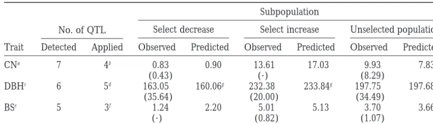
TABLE 2
Comparison of the predicted and observed means of the selected populations
No. of QTL
Subpopulation
Select decrease Select increase Unselected population
Trait Detected Applied Observed Predicted Observed Predicted Observed Predicted
CNa 7 4b 0.83 0.90 13.61 17.03 9.93 7.83
(0.43) (·) (8.29)
DBHc 6 5d 163.05 160.06g 232.38 233.84g 197.75 197.68
(35.64) (20.00) (34.49)
BSe 5 3f 1.24 2.20 5.01 5.13 3.70 3.66
(·) (0.82) (1.07)
CN, DBH, and BS denote cone number, diameter, and branch score, respectively. Numbers in parentheses are standard deviations.
aNumbers of individual trees are 3, 1, and 113 in the three subpopulations. bSelect cone QTL at [2, 6, 0], [5, 10, 0], [10, 5, 7], and [10, 9, 0].
cNumbers of individuals are 2, 3, and 129 in the three populations.
dSelect diameter QTL at [1, 4, 0], [2, 2, 0], [5, 5, 0], [10, 5, 9], and [12, 5, 9]. eNumbers of individuals are 1, 5, and 128 in the three populations.
fSelect branch score QTL at [11, 4, 21], [11, 6, 0], and [12, 5, 0]. gAssume that the QTL at [1, 3, 61] and [1, 4, 0] have coupling phase.
which is a reflection of the positive genetic correlation table in maximization as the number of QTL fitted into
the model increases (HaleyandKnott1992;
Satago-between the two traits. Generally, the estimated and
observed results were quite close based on the MIM pan et al. 1996). We used the method of maximum
likelihood in estimation by applying the general formu-result as found in this sample.
las ofKaoandZeng(1997) to maximize likelihood and
obtain MLEs as well as the variance-covariance matrix
DISCUSSION of the MLEs. The MLEs have some attractive properties,
such as invariance, consistency, and asymptomatic effi-A new QTL mapping approach named MIM is
pro-ciency, in statistical inference. If prior information of posed. It uses multiple-marker intervals simultaneously
parameters is available, the Bayesian approach, such as to construct multiple QTL in the model for QTL
map-in Satagopan et al. (1996) and Sillanpaa and ping. The MIM model is based on Cockerham’s model
Arjas (1998), can be used to incorporate the prior (C-H. KaoandZ-B. Zeng, unpublished results) for
de-information in estimation. By specifying prior density fining genetic parameters and on the general formulas
of parameters, they used Markov chain Monte Carlo to
ofKaoandZeng(1997) for statistical estimation. Using
evaluate the posterior density and to output empirical the MIM model, stepwise and chunkwise selections with
distribution of QTL parameters for QTL mapping. The the LRT statistic as a selection criterion are proposed
MIM approach of using the multiple-QTL model in to identify QTL, to separate linked QTL, and to analyze
QTL mapping distinguishes itself from the current ap-epistasis between QTL. The asymptotic standard
devia-proaches, such as IM and CIM, by the ability to use tions of the estimated QTL positions and effects can be
multiple-marker intervals simultaneously to search the obtained for constructing the C.I.s. With the estimated
chromosome region between markers for QTL. As a QTL effects and positions provided by MIM, the
vari-result, the MIM method may provide greater power ance components of QTL, the heritability of a
quantita-and precision for QTL mapping. However, it should be tive trait, and the genotypic values of individuals can be
noted that the significance level of the multiple-QTL estimated, and marker-assisted selection can be
per-model depends on the marker data structure and the formed for trait improvement. Experimental data on
unknown true model, and the critical value for claiming three traits on radiata pine were analyzed to illustrate
QTL detection becomes a complicated issue for MIM the potential power and benefit of MIM in comparison
(seestrategy of qtl mapping). In the example, we with the current methods, such as IM and CIM. While
used an ad hoc critical value. This value is appropriate a backcross MIM model was used here as an example,
for the one-QTL model, but it may not be appropriate
the MIM model can be easily extended to an F2
popula-for MIM. Although the MIM method claims more QTL
tion (C-H. Kao andZ-B. Zeng, unpublished results).
detection than the current methods in data analysis, it The MIM model is a multiple-QTL model. When the
is not appropriate to conclude that the MIM method is multiple-QTL model is considered, the likelihood is a
1214 C-H. Kao, Z-B. Zeng and R. D. Teasdale
appropriate critical value for the multiple-QTL model epistasis into account without causing a problem in the
backcross population. For tree diameter and cone num-has been solved.
Under the ad hoc critical value, MIM detected six QTL ber, respectively, epistasis contributed 10.38 and 14.14%
of the total genetic variance. Therefore, epistasis should for tree diameter and CIM detected only two of them
on the first linkage group in this example. IM failed to be generally considered in searching for QTL and
marker-assisted selection. For example, in Figure 2a, detect any QTL (Figure 1). The major reason for this
difference is that CIM is not capable of controlling the the best combination of QTL genotype at positions
[2,2,0] and [12,5,9] was AABB, which had an estimated two detected linked QTL simultaneously in further
map-ping. As a result, only the QTL at position [1,4,0] is genotypic value of 13.2. If epistasis was ignored,
geno-type AABb, with estimated genotypic value 1.75, would controlled, but it does not contribute substantially to
reducing the genetic variation because its effect has be selected. The benefit of taking epistasis into account
was reflected in the mapping result in Table 1 and in been canceled out by ignoring the linked QTL with
opposite effects at position [1,3,61]. Accordingly, most grouping genotypes in Table 2.
It has been 76 yr since Sax (1923) associated seed
of the genetic variance (76.75%) contributed by the two
linked QTL becomes part of the genetic residue, making coat characters with seed size in beans. The QTL
map-ping model has evolved from using marker analyses, the other four QTL undetectable. This shows the beauty
of MIM, which allows the current detected QTL being e.g., t -test, simple or multiple regression, to one-QTL
model (IM and CIM), and further to the multiple-QTL fitted directly into the model to search for the next
QTL. Consequently, more QTL were detected by MIM model, such as the MIM approach. In practice, the
tected QTL will be used for selecting parents with de-than the current methods in this example.
In the data analyses, MIM localized two linked QTL sired genotypes for producing progeny or gene transfer
to achieve the ultimate goal of trait improvement in with large opposite directions of effect in the third
inter-val of linkage group 1 (Figure 1a). They contributed later generations. QTL have to be mapped as precisely
as possible to ensure good quality of the follow-up opera-76.75% of the total genetic variance. The size of this
interval was 74.8 cM, so it is suggested that more markers tion on QTL. Therefore, precision and unbiasedness
in estimating the parameters of QTL should be more should be added to this interval to permit further
investi-gation. Two linked QTL, one controlling diameter and important than the ease of computation and
implemen-tation in QTL mapping. The compuimplemen-tation burden of another controlling cone number, were detected in the
same fifth interval of linkage group 10 (Table 1). The the multiple-QTL model is heavy when compared with
the one-QTL model. However, the gain of doing so, as estimated locations are 2 cM apart. Further investigation
is needed to check if they are the same (pleiotropic) shown in this article, could be significant. Although
further work is needed to establish a theoretical basis or different (closely linked) QTL. The likelihood profile
of linkage group 12 in Figure 1e is a result of condition- for determining an appropriate criterion of model
selec-tion in QTL mapping under MIM, MIM has the potenti-ing on the other five unlinked QTL. It shows multiple
significant peaks, which could suggest multiple-linked ality to be more powerful and more precise in QTL
mapping by directly conditioning putative QTL and in-QTL on the same linkage group. However, after further
investigating the linkage group, there was no evidence corporating possible epistasis in the model. Thus, more
genetic variation can be controlled in the model. With of multiple QTL given the peak at position [12,5,9] and
the other five detected QTL. It is therefore concluded the estimates of QTL parameters, other composite
ge-netic parameters, such as the gege-netic variance compo-that there is only one QTL at position [12,5,9] on
link-age group 12. nents and heritabilities, can also be estimated. In
addi-tion, based on the MIM results, genotypic values of Another benefit derived by MIM is that epistasis can
be readily incorporated in the model for analysis or individuals can be estimated to allow desired genotypes
to be selected in marker-assisted selection under various searching for epistatic QTL. When taking both main
and epistatic effects into account in searching for QTL, requirements (e.g., cost, efficiency, and trait
correla-tions). the critical value for hypothesis testing needs to be
ad-justed for the extra degree of freedom for epistasis. It An initial version of the MIM program source code
(written in Fortran 77 language) is available on the is interesting to know that the estimated main effects of
linked QTL are asymptotically unbiased in the backcross worldwide web (http://www.stat.sinica.edu.tw/zchkao/).
A more user-friendly package can be developed based
population (appendix), but they are biased in the F2
population if epistasis is present and ignored in map- on this program. Using the MIM program, we
imple-mented stepwise and chunkwise selections with the LRT
ping (Kao 1995). This is because the coded variables
for main and epistatic effects in Cockerham’s model statistic as a selection criterion to search for QTL in
data analyses. In analyzing the data, we chose the two are still orthogonal under linkage disequilibrium for
the backcross population but not for the F2population. linked QTL with opposite direction of effect on the
first linkage as a starting point to initiate the selection This asymptotic unbiasedness property ensures that
maternal half-sib family and RAPD markers. Genetics 144: 1205–
also tried another possible starting point at [12,5,0] to
1214.
initiate the process and obtained the same final model. Grignola, F. E., I. HoescheleandB. Tier,1996a Mapping
quanti-tative trait loci via residual maximum likelihood: II. A simulation
This final model obtained by model selection might
study. Genet. Sel. Evol. 28: 479–490.
not be optimal. Even though the optimal model was
Grignola, F. E., I. Hoeschele, Q. ZhangandG. Thaller,1996b
obtained, there is no guarantee that it is the true model Mapping quantitative trait loci via residual maximum likelihood:
I. Methodology. Genet. Sel. Evol. 28: 491–504.
(the estimated QTL are the true QTL) for limited
sam-Hackett, C. A.,andJ. I. Weller,1995 Genetic mapping of
quantita-ple size. Ultimately, the reliability of the identified QTL
tive trait loci for traits with ordinal distributions. Biometrics 51:
will depend on further experiments to assess the validity 1252–1263.
Haldane, J. B. S.,1919 The combination of linkage values and the
of QTL. There is no single criterion that plays the role
calculation of distances between the loci of linked factors. J.
of a panacea in the model selection problem. Other
Genet. 8: 299–309.
model selection techniques and criteria could also be Haley, C. S.,andS. A. Knott,1992 A simple regression method
for mapping quantitative trait loci in line crosses using flanking
implemented. It is a very important task to explore and
markers. Heredity 69: 315–324.
automate the model selection procedures of the MIM
Hoeschele, I.,andP. Vanranden,1993a Bayesian analysis of
link-approach for general use in the QTL mapping commu- age between genetic markers and quantitative trait loci: I. Prior
knowledge. Theor. Appl. Genet. 85: 953–960.
nity.
Hoeschele, I.,andP. Vanranden,1993b Bayesian analysis of link-We are greatly indebted to Dr. Chung-I Wu and three anonymous age between genetic markers and quantitative trait loci: II. Com-reviewers for their comments and criticisms. Chen-Hung Kao is grate- bining prior knowledge with experimental evidence. Theor. Appl.
Genet. 85: 946–952. ful to Corinna Lange for her suggestions. C-H.K. was supported by
Jansen, R. C.,1993 Interval mapping of multiple quantitative trait grants NSC87-2313-B-324-001 and NSC88-2313-B-324-001 from the
loci. Genetics 135: 205–211. National Science Council, Taiwan, Republic of China; Z-B.Z. was
Jansen, R. C.,andP. Stam,1994 High resolution of quantitative funded by GM-45344 from the National Institutes of Health and no.
traits into multiple loci via interval mapping. Genetics 136: 1447– 9600645 from the United States Department of Agriculture Plant 1455.
Genome Program. Jayakar, S. D.,1970 On the detection and estimation of linkage between a locus influencing a quantitative trait character and a marker locus. Biometrics 26: 451–464.
Jiang, C.,andZ-B. Zeng,1997 Mapping quantitative trait loci with LITERATURE CITED dominant and missing markers. Genetica 101: 47–58.
Kao, C.-H.,1995 Statistical methods for locating the positions and
Aitken, K. S., G. Smail, J. Drenth, Y. Li, C.-H. Kaoet al., 1997 Detec- analyzing epistasis of multiple quantitative trait genes using mo-tion of quantitative trait loci (QTL) for cone producmo-tion in Pinus lecular marker information. Ph.D. Thesis, North Carolina State
radiata, pp. 337–341 in IUFRO ’97 Genetics of Radiata Pine, edited University, Raleigh.
byR. D. BurdonandJ. M. Moore.Proceedings of NZFRI-IUFRO Kao, C.-H.,andZ-B. Zeng,1997 General formulas for obtaining the Conference, 1–4 December, and Workshop, 5 December, Ro- MLEs and the asymptotic variance-covariance matrix in mapping torua, New Zealand, FRI Bulletin no. 203. quantitative trait loci when using the EM algorithm. Biometrics
Akaike, H.,1974 A new look at the statistical model identification. 53:359–371.
IEEE Trans. Auto. Control 19: 716–723. Kleinbaum, D. G., L. L. KupperandK. E. Muller,1988 Applied
Atkinson, A. C.,1980 A note on the generalized information crite- Regression Analysis and Other Multivariate Methods. PWS-KENT Pub-rion for the choice of a model. Biometrika 67(2): 413–418. lishing Company, Boston.
Carbonell, E. A., T. M. Gerig, E. BalansardandM. J. Asins,1992 Lander, E. S.,andD. Botstein,1989 Mapping Mendelian factors Interval mapping in the analysis of nonadditive quantitative trait underlying quantitative traits using RFLP linkage maps. Genetics
loci. Biometrics 48: 305–315. 121:185–199.
Churchill, G. A.,andR. W. Doerge,1994 Empirical threshold Li, Z., S. R. M. Pinson, W. D. Park, A. H. PatersonandJ. W. Stansel, values for quantitative trait mapping. Genetics 138: 967–971. 1997 Epistasis for three grain yield components in rice (Oryza
Darvasi, A., A. Weinreb, V. Minke, J. I. WellerandM. Soller, sativa L.). Genetics 145: 453–465.
1993 Detecting marker-QTL linkage and estimating QTL gene Lincoln, S. E., M. J. DalyandE. S. Lander,1993 Constructing Ge-effect and map location using a saturated genetic map. Genetics netic Linkage Maps with Mapmaker/Exp Version 3.0. The
White-134:943–951. head Institute, Cambridge, MA.
Dempster, A. P., N. M. LairdandD. B. Rubin,1977 Maximum like- Little, R. J. A.,andD. B. Rubin,1987 Statistical Analysis with Missing lihood from incomplete data via the EM algorithm. Journal R. Data. John Wiley, New York.
Stat. Soc. 39: 1–38. Louis, T. A.,1982 Finding the observed information matrix when
Doerge, R. W.,andG. A. Churchill,1996 Permutation test for mul- using the EM algorithm. J. R. Stat. Soc. Ser. B 44: 226–233. tiple loci affecting a quantitative character. Genetics 142: 284– Miller, A. J.,1990 Subset Selection in Regression. Chapman and Hall,
294. London.
Draper, N. R.,andH. Smith,1981 Applied Regression Analysis, Ed. Satagopan, J. M., B. S. Yandell, M. A. NewtonandT. C. Osborn,
2. John Wiley & Sons, New York. 1996 A Bayesian approach to detect quantitative trait loci using
Dupuis, J.,andD. Siegmund,1999 Statistical methods for mapping Markov chain Monte Carlo. Genetics 144: 805–816.
quantitative trait loci from a dense set of markers. Genetics 151: Sax, K.,1923 The association of size difference with seed-coat pat-373–386. tern and pigmentation in Phaseolus vulgaris. Genetics 8: 552–560.
Geisser, S.,1975 The predictive sample reuse method with applica- Schwarz, G.,1978 Estimating the dimension of a model. Ann. Stat. tions. J. Am. Stat. Assoc. 70: 320–328. 6:461–464.
Gelfand, A. E.,andS. K. Ghosh,1998 Model choice: a minimum Sillanpaa, M. J.,andE. Arjas,1998 Bayesian mapping of multiple posterior predictive loss approach. Biometrika 85: 1–11. quantitative trait loci from incomplete inbred line cross data.
Grattapaglia, D.,andR. R. Sederoff,1994 Genetic linkage map Genetics 148: 1373–1388.
of Eucalyptus grandis and Eucalyptus urophylla using a Pseudo-Test- Stone, M.,1974 Cross-validation choice and assessment of statistical cross: mapping strategy and RAPD markers. Genetics 137: 1121– predictions. I. R. Stat. Soc. B 36: 111–147.
1137. Terasvirta, T.,andI. Mellin,1986 Model selection criteria and
Grattapaglia, D., F. L. G. Bertolucci, R. PenchelandR. R. Sed- model selection tests in regression models. Scand. J. Stat. 13:
eroff,1996 Genetic mapping of quantitative trait loci control- 159–171.