Recognition of Sketch-based Passwords with Biometric Information Using A Generalized Simple K-Space Model.

(1)

ABSTRACT

RIGGAN, BENJAMIN S. Recognition of Sketch-based Passwords with Biometric Information Using A Generalized Simple K-Space Model. (Under the direction of Wesley E. Snyder.)

For many decades, text-based passwords have been the norm for information security. Recently, many have proposed to replace traditional passwords with various types of graphi-cal passwords, such as drawing-based, recognition-based, cue-point based systems. In this work, one such drawing-based, or drawmetric, approach is presented. This proposed method combines both spatial and biometric information at a low level in order to achieve both security and usability (in terms of recognition performance).

The proposed algorithm for recognizing sketch-based passwords is an extension and generalization of a shape recognition algorithm called Simple K-Space (SKS). SKS achieves a sufficient level of performance by accumulating similarity evidence. If enough evidence exists, then the sketches are considered to be similar and access is granted. Otherwise, system access is denied due to insufficient proof of similarity. The algorithm has several advantages over existing methods, including invariance to similarity transformations, robustness to starting and ending points, and fusion of biometric information at a low level.

The novel authentication system, which uses the generalized SKS algorithm, is a semi-supervised system that requires minimal training (3–5 examples per user) during enrollment. While other approaches, such as support vector machines (SVMs), artificial neural networks (ANNs), and hidden Markov models (HMMs), require many exemplars in order to achieve sufficient performance, the generalized SKS approach performs extremely well with few training samples and minimal supervision.

(2)

BioS-ketch databases). The new insights and observations provided include uniqueness of the model, tolerance (or robustness) of the framework, and computational efficiency. Further-more, several experiments are conducted in order to compare performances, study variability due to the human-computer interaction, and provide benchmark performances.

(3)

(4)

Recognition of Sketch-based Passwords with Biometric Information Using A Generalized Simple K-Space Model

by

Benjamin S. Riggan

A dissertation submitted to the Graduate Faculty of North Carolina State University

in partial fulfillment of the requirements for the Degree of

Doctor of Philosophy

Electrical Engineering

Raleigh, North Carolina

2014

APPROVED BY:

H. J. Trussell Edgar Lobaton

Larry K. Norris Cliff Wang

(5)

DEDICATION

(6)

BIOGRAPHY

Benjamin S. Riggan was born in Charleston, S.C., but grew up outside of Raleigh, N.C. From an early age, he exhibited success in math and science. He attended North Carolina State University, first receiving a BS degree in Computer Engineering in December of 2009. While working as an undergraduate teaching assistant, he soon became interested in the fields of computer vision and pattern recognition. He worked on a autonomous vehicle research project headed by his future advisor and mentor, Dr. Wesley E. Snyder.

Continuing his education, Benjamin received his MS degree in Electrical Engineering from North Carolina State University in December of 2011. During his master’s, he studied under the direction of Dr. Wesley E. Snyder. He began working in medical imaging, studying how to detect microcalcifications in mammograms using machine learning and pattern recognition techniques.

His dedication and success under Dr. Snyder, led to funding for PhD from the US Army Research Office. Therefore, continuing his studies under the direction of Dr. Snyder, he will receive his PhD in Electrical Engineering from North Carolina State University in the fall of 2014.

In August of 2014, Benjamin plans on working for the US Army Research Lab as postdoc-toral researcher. He will continue researching in the fields of computer vision and pattern recognition, and hopefully will build a successful career in this area of research. His goals for the future include lifetime learning, state-of-the-art research, and mentoring/teaching

(7)

ACKNOWLEDGEMENTS

I would like to thank committee for their guidance and critical feedback. First, I want to thank my advisor, mentor, and teacher Dr. Wesley Snyder for the time, effort, and dedication he invested into my education and my future. Words cannot express the appreciation I have for the countless lectures, discusses, and even intellectual debates throughout the years. I am truly thankful for the opportunities he gave me. Secondly, I would also like thank Dr. Larry Norris for the many discussions we regarding the mathematical theory surrounding the work in this dissertation. Although, I did not always see where I was going, he was there to point me in the right direction; letting me discover the answers I was seeking on my own. Next, I want to thank Dr. Joel Trussell who has always has inspired me to become a better researcher and instructor. His door almost always open, and he enjoys discussing difficult and challenging problems. Over the years, he has taught me how to provide better self-evaluations of my own work, for the purposes of improvement. I also thank Dr. Edgar Lobaton for his incites and perspectives. He helped me take a step back and see problems in a new light. Last, but not least, I would like to thank Cliff Wang from the US Army Research Office without whom I may have never had the opportunity for pursuing a PhD. I would also like to the thank him for the many career advancement opportunities that he has provided me.

(8)

LIST OF TABLES

Table 2.1 List of local and global features used in handwriting applications. . . 11 Table 2.2 Summary of various HMM approaches for handwriting and character

recognition. . . 15

Table 5.1 Performance comparison between DTW and SKS on DooDB database, which included both doodles and pseudo-signatures. The best perfor-mance is achieved using the SKS-Bio, which is the approach presented in this paper. . . 73 Table 5.2 Performance comparison between the sketch-based password system with

and without biometric pressure. Observe how the pressure makes an im-provement in performance in almost all cases: all skilled forgery scenarios, and the 5 example case for random forgeries. . . 74

Table 6.1 Comparison between Timer and UI based interrupts. . . 78 Table 6.2 A comparison of different ordered interpolations. . . 83 Table 6.3 Summary of model, accumulator, and total computational complexities

using each approach. “Approach 1” precomputes and stores the model, and “Approach 2” does not store the model. . . 87 Table 7.1 Participant demographics. . . 94 Table 7.2 Summary of EER (%) performances using the Fréchet distance and SKS.

(12)

LIST OF FIGURES

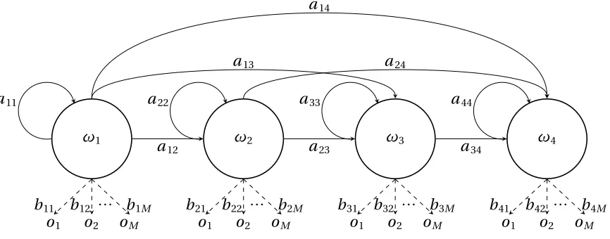
Figure 2.1 Example digitizer and tablet computer for online handwriting recognition 8 Figure 2.2 Example left-to-right HMM. . . 14

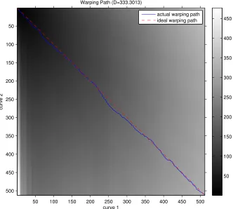
Figure 3.1 The optimal warping path for two signatures are plotted. Thedashedline shows the ideal alignment, and thesolidline shows the actual alignment of the two signatures. The grayscale background at a point(i, j)shows cumulative dissimilarity,D(si,tj), which represents the total dissimilarity

up to aligning theit h_{sample point of}_S_and_jt h _{sample of}_T_{. Notice that}

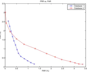
the cumulative dissimilarity increases as the path goes away from the upper left corner of the image, which is expected for twodistinctsignatures. 24 Figure 3.2 Example signatures from SVC databases. . . 27 Figure 3.3 Performance curves for both SVC2004 databases. . . 28

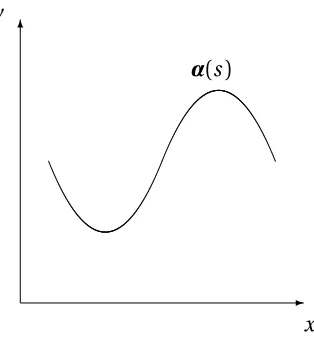
Figure 4.1 A curve in the plane parameterized by arc length. . . 34 Figure 4.2 If the template and test shapes are similar then the accumulator should

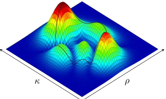
exhibit a significant peak (a). Otherwise, no significant peak should occur (b). . . 37 Figure 4.3 The surface represents the model and the line illustrates an integration

path, which defined by a curve, over the model. Note that the path is not necessarily closed. . . 41 Figure 4.4 The plot shows the average and variation of the entropy for a hand drawn

circle, square, figure 8, and signature. . . 44

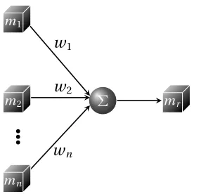
Figure 5.1 The diagram depicts the primary components of both the enrollment and login phases for the proposed sketch-based password system. The inputs (depicted with arrows) to the “Scale Normalization” blocks for both enrollmentandloginrepresent the input sketches from the user for the respective phases. . . 46 Figure 5.2 Computing the representative model for a set of input sketches. The nodes

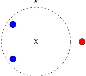
on the left represent the individual models constructed from the input sketches and the output node symbolizes the representative model. . . 52 Figure 5.3 The blue dots represent sketches that are considered inliers,the red dot

represents an outlier, the X represents the representative for the set. The inliers are determined by the predetermined margin of error,". . . 55 Figure 5.4 The surface represents the model constructed over theρ-s feature space

for an ellipse, and the line represents an integration path defined byˆx

and the features ofα`. The result from each integral path represents the

(13)

Figure 5.5 Example of an accumulator that indicates a sketch (shown on top of the accumulator) that is consistent with the model (a), and an accumulator that indicates a different sketch (also shown) is inconsistent with the same model (b). . . 58 Figure 5.6 Shows the interpolation between a heart and a figure-8 (row 1). Then, the

corresponding projections of the models onto theρ-s plane are shown in row 2. Here, we can see that the first two shapes (and models) are more similar than the first and the last. . . 66 Figure 5.7 The plot shows how the MSE in the “space of sketches” is reflected in

the “space of models” for the interpolation from one sketch to 4 differ-ent sketches. Initially, the MSE is null for both because the sketches and models are identical. However, as the sketches become different, the mod-els also become increasingly different which is reflected in the examples shown here. The exact nature of the curve depends on both starting point and ending point in the “space of sketches.” . . . 67 Figure 5.8 The test sketch is overlaid on the accumulator in order to show how the

ac-cumulator changes as the shape is deformed. Notice, how even deformed versions of the same sketch reveal a peak in the accumulator (columns 1–4). However, if the sketch is deformed too much the peak is diminished (column 5). . . 68 Figure 5.9 Set of synthetic sketches: (a) heart #1, (b) heart #2, (c) heart #3, (d) figure-8,

and (e) ellipse . . . 70 Figure 5.10 Comparison of average performance curves using different sets of features

for different levels of jitter. . . 71

Figure 6.1 The illustration shows how the continuous model (a) is sampled in order to produce the discrete model (b). . . 79 Figure 6.2 Osculating circle with radiusr. . . 81 Figure 6.3 Estimation of the osculating circle atqi. The radiusr is shown as the line

between the circumcenterc and the pointqi. . . 82

Figure 6.4 Cubic interpolation of a one parameter function. . . 85

Figure 7.1 Screenshot of the application used to collect sketches from human partic-ipants for the BioSketch Database. . . 90 Figure 7.2 Block diagram of data collection experiment. The experiment consists of

(14)

(15)

LIST OF SYMBOLS

A transition probability matrix for hidden markov models ai j individual transition probability inA

α shape, curve, or sketch α∗ _{unnormalized sketch} αd a discretely sampled sketch

α(i)

d a discrete sketch sample

α` a login sketch

αt a test shape or curve

Accα,αt Simple K-Space accumulator

B observation probability matrix for hidden markov models

B domain interval for pressure b orbα local drawing pressure

bj k individual observation probability inB

C orC0 _{covariance matrix (appendix only)}

C a contour

c class label for hidden markov models

D cumulative dissimilarity (DTW), or a set of input observations (RANSAC) d point dissimilarity (DTW), or number of dimensions (other contexts) dF Fréchet distance

δ(·) a delta function

EorE∗ _{eigenvector (appendix only)}

eore∗ _{eigenvector (appendix only)}

ε threshold (DTW)

" margin of error for inlier (outlier) detection

F feature space (generalized SKS) Fi Fourier coefficient

f usually denotes an arbitrary function (except when denoting frequency) f_α(i) feature (generalized SKS)

G high dimensional feature space (appendix only) g usually denotes an arbitrary function

h smoothing parameter for kernels and density estimators h2 differential entropy (in bits)

I set of inliers (RANSAC) i usually used as an index

j usually used as an index, but in the context of complex numbersj =p−1 K a kernel function

(16)

κorκα local curvature of shape, curve, or sketch

κm a x maximum curvature

L SKS likelihood measure

Ls y m asymmetricSKS likelihood measure

l number of features (DTW)

`f or`b used to denote forward and backward bisecting lines for curvature

esti-mation

λ eigenvalue

M used to denote a number of elements

M space of models

m used to denote a number of elements

mα model (SKS)

mα(i) a discrete model sample ˜

m_α unnormalized model (SKS)

N used to denote a number of elements

Np size of local neighborhood aroundp

n used to denote a number of elements

O Big-O notation

oi observation symbol for hidden markov models

Ω correspondence map or warping path (DTW)

ωi hidden markov model state

P set of model parameters (RANSAC)

P space of sketches

p number of sample points p(·) probability density function

p arbitrary path

Φ non-linear mapping (appendix only)

ϕorϕi model (appendix only)

ψ mapping from the “space of sketches” to the “space of models” Q random subset of observations (RANSAC)

qi denotes a points (used in context of curvature estimation)

R set of real numbers

r radius

ρorρα local Euclidean distance between shape, curve, or sketch and reference point (SKS)

ρm a x maximum Euclidean distance

S signature sequence

S domain interval for arc length

(17)

si local signature feature vector

Σ covariance matrix

σ2

ρ variance corresponding to the Euclidean distance feature σ2

κ variance corresponding to the curvature feature σ2

f(i) variance corresponding to an arbitrary feature

T period (related to frequency)

T signature sequence

Ti so isometric transformation

t time

ti local signature feature vector

τ dummy arc length variable

Θ domain interval for drawing direction

θ orθα local drawing direction for a sketch

U random variable (used entropy definition)

U domain interval for Euclidean distance feature u variable of integration

vorvα feature vector (generalized SKS)

vi discrete feature vector for a discrete sample point of a sketch

wi used to denote a weight factor

x x coordinate

x0₍_t₎_or_x0₍_s₎ _{first x derivative with respect to the parameter}_t _or_s _respectively x00₍_t₎_or_x00₍_s₎_{second x derivative with respect to the parameter}_t _or_s _respectively

x vector representing spatial coordinates

x∗ _{spatial location of peak in the accumulator (SKS)}

y y coordinate

y0₍_t₎_or_y0₍_s₎ _{first y derivative with respect to the parameter}_t _or_s _respectively y00₍_t₎_or_y00₍_s₎_{second y derivative with respect to the parameter}_t _or_s _respectively xi x coordinate of a sample point

yi x coordinate of a sample point

z normalization factor (SKS) zi complex numberxi +j yi

(18)

CHAPTER 1 Introduction

There are many types of authentication systems, all of which may be classified as one of the following types:

1. token-based

2. knowledge-based

3. biometric-based

These systems are based on the following queries:what a user a carries,what a user knows, andwho a user isrespectively. Examples of token-based authentication include: keys, RFID fobs, and ID cards; knowledge-based examples are passwords and PINs; and biometric-based systems use face, fingerprint, voice, and signature recognition.

(19)

A major problem with protecting private information is the assumption that text-based passwords provide a sufficient amount of security. The truth is that more than 3,000 U.S. businesses were victims to cyberattacks in 2013[74], most of which use some form of al-phanumeric password.

In theory, traditional passwords provide a sufficient level of security. However, this as-sumes that the user has created a sufficiently complex password that adheres to specific requirements, such as being random, non-dictionary words, 8–15 characters in length, and including lowercase and uppercase letters, numbers, and special symbols. Text-based pass-words are typically only useful against brute force attacks because thepassword space—the total number of possible passwords—is sufficiently large. Other attacks, such as phishing, spoofing, and shoulder surfing, easily overcome the security measures of text-based pass-words.

There are two unanticipated consequences when using text-based passwords: 1) users completely ignore the security measures, or 2) users breach the security measures (despite adhering to password strength requirements). The first case is typical of many who ignore password protocols whenever possible. Users usually do this because they have one (or two) typical passwords that are easy to remember, but inadvertently insecure. The second scenario is typical of a user that creates a sufficiently complex password, but records his/her username and password either on paper or in a textfile called “passwords.” Therefore, traditional passwords are not necessarily as secure as they claim.

(20)

which does not grant access to anyone, and 2) perfect usability, which grants access to all users. Neither case is desired. Ideally, the only person capable of gaining access should be the genuine user.

1.1 Sketch-based Passwords

In this dissertation, a new authentication approach, which combines a sketch (or drawing) with biometric information as the form of authentication, is presented. A sketch is obtained using a digitizer, tablet computer, or any device with a touch sensitive area for user input. Using a stylus (or finger) a person draws his/her sketch in order to access a secured system, which is either local to the device itself or on a remote system elsewhere.

The advantages of sketches are the following:

• memorability

• security

• reliability

• low cost

(21)

devices are also becoming more affordable, therefore keeping software development costs down.

The randomness due the human-computer interaction makes using a sketch-based system somewhat difficult. There are at least two questions to be answered: How accurate can a user replicate his/her own sketch? How secure are such sketch-based systems? The method used to compare sketches must be robust enough to deal with natural variation from the genuine user and simultaneously be secure enough to reject any forgeries. Thus, there are usability and security concerns with sketch-based passwords, as there are with other authentication systems.

The proposed system utilizes concepts from shape recognition, signature recognition, and biometric systems in order to form a robust and reliable authentication system. This method attempts to alleviate many of the aforementioned concerns. To our knowledge, no other sketch-based or drawing-based system achieves the same performance level as the authentication method proposed in this text.

1.2 Contributions

The main contribution of this dissertation is the authentication system itself, which includes the generalized framework for recognizing sketches with biometric information. Using this framework, additional theory is provided in the application of sketch-based passwords, including: computational complexity and the security/usability tradeoff. Additionally, we

(22)

when used with sketch-based passwords. Lastly, we study the human-computer interaction process for sketch-based passwords.

1.3 Summary of Results

The major results presented in the latter chapters of this work are the following:

1. 0.0% equal error rate (EER) on a set of synthetic shapes

2. 1.4% EER (random forgeries) and 28.0% EER (skilled forgeries) on “doodle” or sketches from the DooDB database[68]without biometrics

3. 1.6% EER (random forgeries) and 23.3% EER (skilled forgeries) on pseudo-signatures from the DooDB database[68]without biometrics

4. 0.0% EER (random forgeries) and 3.3% EER (skilled forgeries) on a set of hand drawn sketches

5. 1.74% EER (random forgeries) and 16.75% EER (skilled forgeries) on the BioSketch database

The termsrandomandskilledforgeries will be discussed in detail in Section 7.1.2.

These results demonstrate the effectiveness of the approach on a variety of datasets, multiple users (genuine and forgers), and under many conditions. Refer to the main text for complete details regarding each experiment.

1.4 Organization

(23)

Chapter 2 provides a summary of major literary works related to sketch-based passwords. This literature review provides an overview of handwriting recognition, alternative graphical-based passwords, and biometric systems. The topics discussed in this section provide a solid foundation for the remaining chapters.

Next, signature recognition (Chapter 3) and shape recognition (Chapter 4), which are the most relevant topics when discussing sketch-based passwords. In these two chapters, two approaches: Dynamic Time Warping (DTW) and Simple K-Space (SKS), which are state-of-the-art pattern recognition methods, are discussed in detail. Chapter 4 also introduces a generalized framework which is essential for the approach used for recognizing sketch-based passwords.

Chapter 5 introduces the novel sketch-based authentication system. This chapter is the core of the work presented in this dissertation. Here, the major components of the sketch-based password system are discussed. Additionally, new theory regarding the efficiency, security, and usability is proven, and experimental results are provided to support this theory. Chapter 6 discusses many practical considerations with a discrete implementation, in-cluding sampling, feature estimation, and interpolation. Also, the memory usage versus speed tradeoff is discussed. Understanding this tradeoff is useful for knowing how best to implement a sketch-based password system on servers, desktop or laptop computers, and tablet computers.

Chapter 7 discusses the construction of the Biometric Sketch database or “BioSketch” database. Using sketches from the database, a human factors analysis is performed. This study aims to analyze the variability of sketches provided by genuine users and forgers (skilled and unskilled). Additionally, benchmark performances are provided for the database.

(24)

CHAPTER 2 Background

2.1 Handwriting and Character Recognition

Handwriting recognition and handwritten character recognition are two topics that ulti-mately led to current research problems involving human-computer interactive processes, such as gesture, signature, and drawing recognition. Handwriting recognition consists of many different forms, including handwritten print or cursive[59, 70], different written lan-guages (e.g. Chinese[64, 105], Arabic[40], and Latin[80]), characters[15]or numbers[23], and even context specific handwriting recognition (e.g. dates and checks[46]).

(25)

which is designed to be used with a laptop or desktop computer, uses a separate computer screen for user feedback; this may adversely affect the user experience. Other digitizers and tablet computers overlay the active surface (i.e. touch sensitive screen) on top of the screen for user feedback.

Offline systems, instead, use a camera or scanner to obtain digital image of the handwrit-ing for recognition purposes. Offline systems are not only different from online systems in hardware but also in the type of features used. For instance, the dynamics of handwriting are usually unknown for offline systems.

(a) Wacom Intuos digitizer. Image obtained from [1]

(b) Samsung Galaxy Note 10.1 tablet computer. Image obtained from[2]

(26)

This work primarily focuses on online systems, however, the primary recognition com-ponents of offline systems are similar to those of online systems, after the handwriting is captured and preprocessed. Most handwriting and character recognition systems include the following stages: (1)feature extractionand (2)classification.

2.1.1 Feature Extraction

There are an innumerable number of features used for handwriting recognition; only a subset of features are introduced in this section. Many online systems use a Fourier descriptor as a set of features, and other offline/online systems use spatial or temporal features.

Fourier descriptors generally assume that a given contour is closed. Note that there are existing methods for closing contours[62], as well as extended Fourier descriptor methods for open contours[25].

There are multiple Fourier descriptors that may be used for character or handwriting recognition (see[65]), including:

• complex Fourier descriptor[71]

• affine-invariant Fourier descriptor[7]

• moment-invariant Fourier descriptor[10]

The complex Fourier descriptor is the only feature transform discussed since affine and moment invariant formulations use the same fundamental principle, except for the modification to achieve the desired invariances.

Letnsample points along a given contourC be represented by the complex1_coordinates:

zi =xi+j yi,

(27)

where the pair(xi, yi)represents the planar coordinates theit h contour sample.

Then, the descriptor is represented by the set of Fourier coefficients:

Fi = n−1 X

k=0 zkexp

−j2πi k

n

fori =0 . . .n−1.

Fourier descriptors not only provide a useful descriptor for handwriting recognition; they have a meaningful interpretation. The set of Fourier coefficients,{Fi}n_i₌−₀1, describes

compo-nents of the contour in the frequency domain. Fourier descriptors possess a relationship to transformations in the spatial domain, which are described as (see[97]):

• Scaling (in the spatial domain) produces Fourier coefficients that have all been multi-plied by a constant

• Planar Rotation produces phase shifted Fourier coefficients

• Translation produces Fourier coefficients with a DC (i.e. zero frequency component) offset

These properties allow for invariance to rigid transformations of contours. For additional invariances, refer to[7, 10].

As mentioned previously, Fourier descriptors are not the only features used for hand-writing recognition. Table 2.1 provides a variety of features that have been used in such applications.

(28)

Table 2.1: List of local and global features used in handwriting applications.

Type Feature Description

Global

Time The total time required to write[39, 53] Bounding Box The total writing area required[58]

Pen Ups The total number of times a user lifts up the pen (or finger ) while writing[39]

Pen Downs The total number of times a user presses the pen (or finger) tip down[39]

Local

Position The x and y coordinates of each sample point, typically with respect to some refer-ence[82]

Displacement The difference in x,∆x, and the difference in y,∆y, between sample points[50, 58] Velocity The instantaneous rate of change in position

with respect to time[53, 82]

Acceleration The instantaneous rate of change in velocity [43, 53, 82]

Pressure The point-wise amount of force applied at the pen (or finger) tip by the user in the pro-cess of writing[33, 43, 82]

Curvature The point-wise measure describing the amount of deviation from a line, which is commonly used to model shape[50]

Azimuth The angle between the pen’s projection on the table and the tablet’s coordinate refer-ence angle[33]

(29)

2.1.2 Classification

Constructing a robust and invariant descriptor is one step, but recognizing or classifying them is another. Although there exist many different methods for recognizing handwriting using a feature representation, Hidden Markov Models (or HMMs) are commonly used for this purpose[3, 47, 48, 66].

The primary concepts for HMMs are briefly discussed here, and then a few HMM struc-tures used in handwriting recognition applications are reviewed.

HMMs are widely used in both speech recognition [81]and handwriting recognition [3, 47, 48, 66]applications. A HMM is analogous to theurn-and-ballexperiment[83], in which there areN urns (or vases) each containingM different colored balls. In this experiment, the urns are placed behind a curtain and a person chooses a sequence of urns, according to some random process, pulling one ball from each urn out from behind the curtain at time.

Similarly, a HMM hasN unobservableorhiddenstates (where each state corresponds to an urn), which are denoted{ω1, ω2, . . . , ωN}. The transition sequence between states is

determine by a matrix of transition probabilities

A=          

a11 a12 · · · a1N

a21 a22 · · · a2N

..

. ... ... ... aN1 aN2 · · · aN N

          ,

and the probability of observing a particular observation variable (or colored ball) from the set of possible observations,{o1, o2, . . . ,oM}, is defined within each state. The probability of

observing thekt h_{variable (or symbol) from the}_jt h _{state is denoted by}_b

(30)

observation probabilities is denoted by theN×M matrix B=          

b11 b12 · · · b1M

b21 b22 · · · b2M

..

. ... ... ... bN1 bN2 · · · bN M

         

The urn-and-ball experiment provides a good illustration of a HMM, but how are they used for handwriting recognition (or any other pattern recognition problem)? There are two problems to consider: (1) the evaluation problem and (2) the learning problem.

The goal of the evaluation problem is simply to determine the probability that a given sequence of observations,O, was generated by the HMM, which assumes that the transition and observation probabilities,AandBrespectively, are known. That is, the goal is to compute Pr(c|O,A,B), which represents the probability that the observation belongs to some classc given observation and the HMM with known parametersAandB.

The purpose of the learning problem is to update the HMM probabilities,AandB, based on a collection of known observation sequences (presumably belonging to some classc). The only assumption for the learning problem is the basic structure—the number of states (and/or transitions) and observation symbols—of the HMM. The probabilities for the given

HMM are updated using theforward-backwardalgorithm[30].

The forward-backward algorithm, unlike artificial neural networks (ANNs) and sup-port vector machines (SVMs), doesnotseek an optimal solution for the HMM parameters, however, because this algorithm is a generalization of Expectation-Maximization (EM) an acceptably “good” solution may be obtained.

(31)

ω1 ω2 ω3 ω4 a14

a13 a24

a12 a23 a34

a11 a22 a33 a44

· · ·

o1 o2 oM

· · ·

o1 o2 oM

· · ·

o1 o2 oM

· · ·

o1 o2 oM

b11 b12 b1M b21 b22 b2M b31 b32 b3M b41 b42 b4M

Figure 2.2: Example left-to-right HMM.

theleft-to-right[47]HMMs (Figure 2.2), which prohibit any backward transitions (i.e.ai j =0

forj <i). There is also a subset of left-to-right HMMs that prevent the skipping of any state, meaning that from any single state,ωi, there are only two possible transition: the same state

(ωi) or the next state (ωi+1).

Many have used HMMs for handwriting recognition and achieved varying levels of performances. A summary of the different HMM approaches are presented in Table 2.2. The table shows that there are numerous ways to implement a HMM for handwriting recognition, including word, character, or subcharacter models and different training methodologies.

2.2 Graphical Passwords

Graphical passwords are not new (in fact the idea has been around for quite sometime), but there are still many questions regarding their security and reliability. Graphical passwords belong to one of the following taxa (according to[28]):

(32)

2. Cognometric—recognition-based methods (also referred to as search metric[84])

3. Locimetric—cued-recall based methods.

Table 2.2: Summary of various HMM approaches for handwriting and character recognition.

Author(s) Structure Training Performance

Hu et al.[47] left-to-right without state skipping

“nebulous stroke models”— subcharacter model (3100+ samples)

~3.1% error (~1600 test samples)

Rigoll et al.[88] left-to-right without state skipping

character model (1640 sam-ples)

0.65% error (single characters) and 30% error (word recognition) Martin et al.[67] left-to-right character model with Baysian

Information Criterion (BIC) for optimal number of states

6% error (discrete

HMM) and 0%

error (continuous HMM)

Drawmetric systems require users to construct a unique sketch or drawing as a password. This construction is referred to as theenrollmentphase. Then, atlogintime genuine users are expected to recall and accurately reproduce the password. This type of system requires that a user physically draw a “password” using a digitizer or tablet, which is a noisy process itself. However, prior to drawing, the user must recall the sketch from memory (including the associated biometric properties, e.g., pressure). Then, the user must convert that depic-tion into a sequence of muscle movements to physically reproduce the drawing. Therefore, drawing a sketch-based password requires a complex human-computer interaction.

(33)

the way for success and acceptance of drawmetric application.

Probably, the most notable drawmetric system is Draw-A-Secret (DAS)[52]. The DAS approach uses a coarse grid, which is displayed to the user, to encode the drawing. The drawing is encoded using the grid cells. The ordered sequence of grid cells that the drawing enters produces a password string. Thus, the matching procedure for DAS is virtually no different from text-based passwords (except for the fact that the string is generated from a drawing); the string produced at login time is compared with the string stored during enrollment.

There are some extensions to DAS which have improved performance. For example, Background Draw-A-Secret[32]improves performance by adding background images. Yet Another Graphical Password (YAGP)[37]improves performance by using a finer grid than the original DAS approach. By removing the visible grid for drawing and including stroke color as an additional feature, Passdoodle[38, 99]improves performance.

One drawback to DAS and similar approaches is the difficulty of encoding near inter-section points of grid cells. To alleviate this problem, the Pass-Go[98]approach uses grid intersection points as anchor points instead. Thus, the encoding records an ordered sequence of horizontal, vertical, and diagonal strokes.

(34)

mouse, keyboard, or touch screen.

The best example of a recognition-based system is PassFaces[78]. During enrollment, the user is presented with a random set of faces and asked to select a subset of them as a “password.” At login time, the user is presented with the correct set of faces dispersed among

a random set of other faces. The user is then asked to identify the correct set of faces. Instead of faces, the Déjà Vu[29]system uses a set of images with graffiti-like patterns and artwork. Studies[27, 85]have shown that, even with choosing faces, people are predictable in their choice of password. Predictability in security implies that the entropy, or measure of randomness that is related to “security,” is reduced. Déjà Vu attempts to alleviate this problem by making the images very randomized, so that a bias or preference does not exist toward any particular image.

Locimetric systems, instead of requiring users to remember entire images, have users recall and identify specific points or regions within an image. The idea is to reduce the amount of information that a user is required to remember. Given a larger image, a user selects an ordered sequence of points or regions located within the image. In principle, the image should help stimulate the process of remembering the points previously chosen, hence the term cued-recall.

The most prominent cued-recall based method is PassPoints[100, 101, 102]. PassPoints presents the user with a single image—typically having numerous landmarks: people, build-ings, objects, etc.—in which during enrollment the users is supposed to select 5 different locations. At login time, the user is again presented with the same image, and the user must chose the correct set of points within the image in precisely the same order.

(35)

one point is incorrect, access is denied.

Many of the methods using drawmetric, cognometric, and locimetric password systems are compared and contrasted in[16]. This literature survey analyzes the multitude of methods in terms of both usability and security, especially the vulnerabilities to different attacks (e.g. brute force, phishing, and shoulder surfing).

2.3 Biometric Systems

Biometrics systems—systems that measure and analyze certain biological properties for the purposes of identity recognition [36]—are steadily becoming a part of everyday life, including in commercial access systems, personal computers, and smart phones. Biometrics are increasingly popular because they are supposed to be universal, distinct, permanent, and collectable[51]properties that uniquely identify an individual. For these reasons, biometrics are considered much more secure than traditional passwords.

Biometrics include biological properties such as fingerprints, voices, faces, and even handwriting. Fingerprints have been widely used and accepted in forensic, commercial, government security, and consumer applications. Despite the fact that fingerprints are known to be unique to every individual, there are still concerns in terms of a system’s ability to recognize fingerprints (especially with consumer applications). For example, fingerprint recognition is very sensitive to noise and occlusion. In most cases, the signal-to-noise ratio (SNR) is low, which increases the difficulty of recognizing fingerprints accurately (implying the possibility of a breach in security).

(36)

fingerprint including varying poses and pressure.

Voice recognition systems, although not as widely used in security application, are used applications such as voice-to-text in cars and smart phones, and voice command systems. There are many reliability concerns when it comes to voice recognition systems for user authentication. Multiple variables, such as distance to microphone(s), background noise, and vocal anomalies (e.g. colds, dialects, and accents), affect the reliability of a voice recognition system. The most concerning of these are the anomalies because they naturally occur to human voices, but voice recognition systems still experience difficulty in handling these effects.

Facial recognition systems for authenticated access are also becoming more common because of advancements with this technology. However, there are still concerns about the reliability of these systems. Facial recognition most commonly experiences difficulties with occlusion. Faces can be occluded because of clothing or accessories, lighting conditions, or even pose. As with fingerprints, the confidence of the face recognition is reduced when there is occlusion. Under normal operating conditions, one would expect facial recognition to perform quite well. However, there are legitimate security concerns with false acceptances— when the system grants access to an unauthorized person.

(37)

(38)

CHAPTER 3 Signature Recogntion

Before discussing the recognition problem associated with sketches, it is necessary to discuss the related problem of signature recognition. Signatures may be viewed as a special type of sketch; one with high complexity and high intra-class variance. This special case is one that has been widely studied.

(39)

in a way such that the dissimilarity between two signatures is minimized. After optimizing, if the dissimilarity is sufficiently small then the signatures are considered to be the same. Regional correlation approaches to signature recognition also look for correspondences. Instead of using singular points on the signature (like DTW), local regions (i.e. segments) are used to determine correspondence. Using a correlation measure, the cross-correlation of two signatures results in a correlation for each segment. Then, an average correlation is used to determine signature similarity.

Machine learning techniques, like hidden Markov models (HMMs)[30, 103]and artificial neural networks (ANNs)[57, 58]have also been applied to signature recognition. HMMs approach signature recognition from the random process perspective—the goal is to con-struct a stochastic model capable of generating class of signatures with high probability. A HMM is a fixed state machine with some number of states, transitions, and observations (from a defined vocabulary). Using a set of known signatures from the same class, the model can be trained. By training, it is implied that the state transition probabilities are iteratively updated (with the hope of generalizing the model). Then, a signature from an unknown class is compared against the model, by determining the likelihood that the given HMM (with known probabilities) will generate that particular signature. If the likelihood is sufficiently large (which implies some type of thresholding), then the signature belongs to the same class as the ones used to train the model.

(40)

depends on the assumptions used.

3.1 The Correspondence Problem

A common problem that many signature recognition method attempt to solve is the corre-spondence problem—the problem of finding corresponding or matching points, typically, in

presence of noise and arbitrary transformations (temporal and spatial). In most cases, the correspondence problem refers to determining which regions of one image match those of a second image, where the second image is produced from the spatial displacement of the camera or objects in the field of view or a time lapse. However, for signature recognition, this problem means determining which points/regions of the signature match those of another signature.

Under ideal conditions, solving the correspondence problem is trivial. However, under general deformations and noise caused by a random process, e.g. a signature or handwriting process, finding correspondences proves to be more difficult. This is because under severe perturbations the unique features or properties of a signature may appear to vanish. Thus, the detection of correspondences is more difficult.

One approach that attempts to find an optimal alignment (i.e. correspondence) of two signatures for comparison is DTW. This method is discussed in more detail below.

3.2 Dynamic Time Warping

The goal of DTW is to the find the correspondence map,Ω, which can be graphed using a grid (Figure 3.1), that minimizes the total dissimilarity between two signatures,S= [s1s2 · · ·sn]

(41)

Warping Path (D=333.3013)

curve 1

curve 2

50 100 150 200 250 300 350 400 450 500

50

100

150

200

250

300

350

400

450

500

actual warping path ideal warping path

50 100 150 200 250 300 350 400 450

Figure 3.1: The optimal warping path for two signatures are plotted. Thedashedline shows the ideal alignment, and thesolid line shows the actual alignment of the two signatures. The grayscale background at a point(i, j)shows cumulative dissimilarity,D(si,tj), which

represents the total dissimilarity up to aligning theit h _{sample point of}_S_and_jt h _{sample of}_T_.

Notice that the cumulative dissimilarity increases as the path goes away from the upper left corner of the image, which is expected for twodistinctsignatures.

T= [t1t2· · ·tm](anl ×m matrix). The cumulative dissimilarity by aligning theit h point ofS

with thejt h _{point of}_T_is

D(si,tj) =min

α {D(si−1,tα)}+d(si,tj) (3.1)

where d(si,tj)is the additional cost associated with aligning samples i and j (usually a

(42)

Equation 3.1 is minimizing the cumulative dissimilarity, over allαsuch that the pointtα

aligns with the pointsi−1. Using recursion, and thus determining the set of corresponding points (not necessarily one to one correspondence), the cumulative dissimilarity between the signatures is then determined by the valueD(sn,tm). Note, that this dissimilarity has never

been shown to be a metric because no proof exists that it satisfies the triangle inequality. All other properties required to be a metric are satisfied. However, in[20]it is shown that the triangle inequality is not violated in a large (on the order of 15 million) set of speech patterns. Therefore, if DTW is shown with statistical validation tolooselysatisfy the triangle inequality then it can approximately be considered as a metric.

Two signatures are considered to match if and only ifD(sn,tm)< ε, where εis some

experimentally determined threshold on the total dissimilarity. Otherwise, the signatures are too different to be considered a match.

The algorithmic complexity of DTW isO(n2₎_[₃₉_]_{. However, this is typically a worst case} scenario. This complexity is alleviated some by use of global and local constraints. Typical constraints include:

Boundary Conditions Typical boundary constraints include the alignment ofs1witht1, and sn withtm.

Monotonic Conditions Assuming theit h _and_jt h _{points are aligned, then point}_i₊_{1 must}

be aligned with a pointk≥j.

Global Path Conditions This restricts the warping path from going to far away from the ideal path.

(43)

two points on the correspondence path are desired over others, then the slope weights are added in the cost function.

3.3 Experiments and Results

In this section, an experiment using DTW for signature recognition is conducted, and the corresponding results are reported.

TheSignature Verification Competition(SVC2004) databases[104]are used to test a DTW algorithm. Examples from each database are shown in Figure 3.2. Both databases include 20 genuine signatures and 20 forgery signatures for 40 different individuals. This experiment examines only the skilled forgery case because it is the more difficult and interesting situation.

The experiment is as follows:

For every user, each genuine signature is compared (using DTW) to every other signature for that user (both genuine and forgery). If a genuine signature is considered too dissimilar, then it is counted as a false rejection. Likewise, if a forgery is considered similar enough, then it is counted as a false acceptance. Performance for most signature recognition (and biometric systems) is measured by the false acceptance rate (FAR) versus false rejection rate (FRR) curves. In some cases, performance is reported in terms of the equal error rate (EER), which is the rate where the FAR and FRR are equal.

(44)

(a) Database 1 SVC2004.

(b) Database 2 SVC2004.

(45)

0 0.5 1 1.5 2 2.5 3 3.5 0

0.5 1 1.5 2 2.5 3 3.5

FRR vs. FAR

FAR (%)

FRR (%)

Database 1 Database 2

Figure 3.3: Performance curves for both SVC2004 databases.

3.4 Discussion and Analysis

The extension of DTW to recognize sketches (rather than signatures) is not a difficult one. However, there are two potential problems with the DTW approach: 1) start/end point dependence and 2) efficiency/generalizability. The assumption that a user starts and ends

at the sameexactlocations when drawing a sketch (or signature) is not a good one. DTW assumes that the starting point of a sketch is best aligned with the starting point of another sketch, and likewise the end point of a sketch is best aligned with the end point of another sketch. However, this is frequently not the case due to user variability in start/end points.

(46)

(47)

CHAPTER 4 Shape Recognition

4.1 What is Shape?

Probably the most distinctive difference between two dissimilar sketches is captured by their shape. The earliest studies of shape theory are found in[18, 19, 54, 108]. These early works led to Kendall’s shape space. Kendall defines shape to be “what is left when the differences which can be attributed to translations, rotations, and dilatations have been quotiented out”[55]. Much research has been performed in the area of shape recognition and shape matching. There are many varied approaches used for differentiating the detailed differences between shapes, including (but not restricted to):

1. Fourier Descriptor methods

2. Statistical methods

(48)

4. Shape matrix and other methods

4.2 Fourier Descriptors

Fourier descriptor methods, such as[8, 79, 106], are appealing for matching curves and shapes because of the invariances to similarity transformations: translation, rotation, and scale. Also, Fourier descriptors exhibit a useful inverse property in which a shape may be reconstructed from the descriptor. The complete descriptor has an infinite number of co-efficients, but truncating to a sufficiently large number of coefficients produces minimal error between the original curve and the reconstructed curve. As the number coefficients is reduced, the corresponding curve becomes smoother, and less similar to the original.

4.3 Statistical Methods

Many statistical shape models exist for shape recognition, including methods using kernel density estimation[89], principle components analysis (PCA)[97], kernel PCA (or KPCA) [92], and shape context[13]. Density estimators use a probabilistic representation of shape, and the similarity between shapes is determined by likeness of the distributions. An ap-proximation of the distribution is determined from a collection of points,{xi}ni=1, which are unordered since shapes do not explicitly have any parameterization. Intuitively, these points are blurred using a kernel (e.g. Gaussian)[95]

K

_x−_x

i

h

(49)

The kernel used to estimate the shape distribution usually includes some form of a smoothing parameter,h, that provides a trade-off between accuracy and smoothness of the distribution.

PCA (KPCA) is a method which computes the dominant linear (nonlinear) directions of maximum variance. PCA methods provide a compact and invariant representation of shape, which are typically used to discriminate dissimilar shapes. PCA works by determin-ing a different coordinate system, which is more representative of the shape distribution. This coordinate system is defined by a set of orthonormal axes that are determined by the principle eigenvectors of the data covariance matrix. KPCA also defines a set of orthonor-mal axes in order to define a new coordinate system. However, the difference is that KPCA does not operate in the input space (like PCA). Instead, the input is mapped nonlinearly to higher dimensional space, and classic PCA is performed in this space. Therefore, when the orthonormal axes in the higher dimensional space are mapped back into the input space, the principle directions are nonlinear. In either case, the coordinate system is used to construct a more compact representation which can discriminate dissimilar shapes. For more detail regarding PCA and KPCA, refer to Appendix B.

(50)

4.4 Accumulation Methods

Accumulation methods, like the Hough Transform[9], have been applied to various shape recognition applications including recognizing lines, circles, and ellipses[14]. In[60] an accumulation technique is used to recognize arbitrary shapes by use of the Simple K-Space algorithm (Section 4.6). The subject of this dissertation is primarily an extension and analysis of this method, which is applied to the recognition of sketch-based passwords.

4.5 Shape Matrix and Other Methods

One important representation of shape is Kendall’s shape matrix[56], which considers shape to be a property that is invariant to rigid transformations. Kendall’s approach to shape first defines apre-shape, which accounts for any translations or changes in scale (or size). Then, shape is considered to be an equivalence class of pre-shapes (represented by the shape matrix), defined by rotations fromSO(n).

A review of multiple shape representations is provided by Zhang and Lu [107]. This review discusses metrics, such as the Hausdorff distance[12, 90], used for comparing shapes. Complex methods using invariant moments[49]and the shape matrix[56]are also described. Lastly, scale space implementations, in particular curvature scale space (CSS)[4, 31]methods, are also used for shape recognition.

4.6 Simple K-Space

(51)

this section only the one parameter method is relevant to the application of shape recognition (and the similar application of sketch-based passwords).

While SKS is an accumulation-based approach, there are some similarities between SKS and Kendall’s[56] perspective on shape. Kendall first constructs a translation and scale invariant representation, and then considers a similar shape to be any rotation of that representation. SKS, however, construct a translation and rotation invariant model, and then considers a similar shapes to be a scaled (or zoomed) version of that model.

-6

x y

α(s)

Figure 4.1: A curve in the plane parameterized by arc length.

The single parameter SKS algorithm begins by constructing a model (i.e. a template) of a given shape in thex-y plane (Figure 4.1). A shape is defined asα(s) = [x(s)y(s)]T_{, where the}

shape is parameterized by a single parameters—arc length (Equation 4.1). Note that shapes are not parameterized explicitly, however, we provide a parameterization in order to compute features necessary for constructing a model that is independent of the parameterization.

s(t) = Z t

t0

(52)

Using a curve, two new shape functions are computed (or estimated),ρα(s)andκα(s), where

ρα(s) =kα(s)−x0kandκα(s) =|α00(s)|is defined as the local curvature at an arc lengths. The

distanceρ_α(s)is with respect to an arbitrary, but constant, spatial reference point,x0. In practice,x0is chosen to be the centroid of the curveα(s). For now, curvature is assumed to be continuously defined over the entire curve, except for points of discontinuity (e.g. endpoints). There are some caveats when using and computing curvature, which are is discussed in Section 6.4 along with details regarding curvature estimation.

Typically,ρα(s)∈ Uandκα(s)∈ K, whereU ⊂Rdefined by[0,ρm a x]andK ⊂Rdefined

by[0, κm a x].ρm a x andκm a x are determined, in practice, by the length of diagonal of the

image plane and the resolution (or sampling rate) of the curve (see Chapter 6) respectively. After computingρ_α(s)andκ_α(s), the model of a curve,α(s), may be computed using the following function:

mα(ρ,κ) = 1 z

Z 1

0

exp −(ρ−ρα(s))

2

2σ2

ρ

!

exp

−(κ−κα(s))

2

2σ2

κ

ds (4.2)

wherez is a normalization factor (see Section 4.8.3),σρandσκare independent smoothing

parameters, ands ∈[0, 1]without loss of generality. The smoothing parameters,σρandσκ,

are usually chosen experimentally. As a rule of thumb,σρandσκare 5%–20% ofρm a xand

κm a x respectively.

The model function,m_α:U × K →R, is a scalar function defined for all ordered pairs

(ρ,κ), and the valuemα(ρ,κ)represents alikelihoodthat there exists a point on the curve that is a distance ofρfrom the reference and has a curvature ofκ. If normalized such that R R

(53)

In fact, Equation 4.2 resembles a kernel density estimator[89]:

p(x) = 1

hd

Z 1

0 K

x−x(τ)

h

dτ

The goal of constructing a model is to determine the similarity between two curves. The matching process for the SKS algorithm implements an accumulation technique[9]to determine theconsistencybetween a shape and model. This consistency measure is used to infer similarity between the shapes.

Given a test curve,αt(s) = [xt(s)yt(s)]T (with curvature functionκαt(s)), theconsistency

ofαt(s)withmα(ρ,κ)is computed using an accumulator (Equation 4.3).

Accα,αt(ˆx) =

Z 1

0

mα(kxˆ−αt(s)k,καt(s))ds (4.3)

In principle, the accumulator represents a likelihood that the pointxˆ= (ˆx,yˆ)is the refer-ence point of a curve,αt(s), that is consistent with the model. If the curve being compared to

the model is the sufficiently similar, then by computing Accα,αt(ˆx)for allxˆ, a sharp peak will

occur at the “best” reference point. Otherwise, the accumulator will not exhibit any signifi-cant peaks. Figure 4.2 illustrates the difference between anidealaccumulator indicating a matching shape and one indicating no match.

4.7 Generalized Simple K-Space

In this section, the 2D SKS model (Section 4.6) is extended to a model with an arbitrary number of dimensions. In many applications, it may be necessary to model more than simply shape (e.g. direction, order, velocity, acceleration, and etc.).

(54)

x

y

(a) Ideal matching accumulator.

x

y

(b) Ideal non-matching accumulator.

Figure 4.2: If the template and test shapes are similar then the accumulator should exhibit a significant peak (a). Otherwise, no significant peak should occur (b).

Now, consider this to be a vector-valued function (still parameterized by arc length). In the 2D case, the function isvα(s) = [ρα(s)κα(s)]T. If the function includesρα(s)and n other functions ofs (associated with the curve), then the vector-valued function is

vα(s) =ρα(s)f_α(1)(s)· · ·f_α(n)(s)

T

.

Fromv_α(s)and Equation 4.2, the generalized model becomes

mα(v) =1 z

Z1

0 exp

−1

2(v−vα(s))

T_Σ−1₍_v

−vα(s))

(55)

where Σ=           σ2

ρ 0 · · · 0

0 σ2_f(1) · · · 0

..

. ... ... ...

0 0 · · · σ2

f(n)

         

The covariance matrix,Σ, is diagonal because the features,ρ_α f_α(1) . . . f_α(n), are all assumed to be independent. In general, feature dependency must be considered. The model,m_α:F →R,

is defined for allv∈ F, whereF ⊂Rn+1.

Then, matching is, again, performed by computing the accumulator. Similar to Equa-tion 4.3, the accumulator is

Acc_α,αt(ˆx) =

Z 1

0

m_α(kxˆ−αt(s)k, f_α(1_t)(s),· · ·, f_α(n_t)(s))ds (4.5)

Recognition of Sketch-based Passwords with Biometric Information Using A Generalized Simple K-Space Model.

ABSTRACT

DEDICATION

BIOGRAPHY

ACKNOWLEDGEMENTS

TABLE OF CONTENTS

LIST OF TABLES

LIST OF FIGURES

LIST OF SYMBOLS

CHAPTER 1

Introduction

1.1

Sketch-based Passwords

1.2

Contributions

1.3

Summary of Results

1.4

Organization

CHAPTER 2

Background

2.1

Handwriting and Character Recognition

2.1.1

Feature Extraction

2.1.2

Classification

2.2

Graphical Passwords

2.3

Biometric Systems

CHAPTER 3

Signature Recogntion

3.1

The Correspondence Problem

3.2

Dynamic Time Warping

3.3

Experiments and Results

3.4

Discussion and Analysis

CHAPTER 4

Shape Recognition

4.1

What is Shape?

4.2

Fourier Descriptors

4.3

Statistical Methods

4.4

Accumulation Methods

4.5

Shape Matrix and Other Methods

4.6

Simple K-Space

4.7

Generalized Simple K-Space

x

y

x

y