Getting More from Segmentation Evaluation

Getting More from Segmentation Evaluation

Martin Scaiano

University of Ottawa Ottawa, ON, K1N 6N5, Canada

[email protected]

Diana Inkpen

University of Ottawa Ottawa, ON, K1N 6N5, Canada

[email protected]

Abstract

We introduce a new segmentation evaluation measure, WinPR, which resolves some of the limitations of WindowDiff. WinPR distin-guishes between false positive and false nega-tive errors; produces more intuinega-tive measures, such as precision, recall, and F-measure; is in-sensitive to window size, which allows us to customize near miss sensitivity; and is based on counting errors not windows, but still pro-vides partial reward for near misses.

1 Introduction

WindowDiff (Pevzner and Hearst, 2002) has be-come the most frequently used measure to evalu-ate segmentation. Segmentation is the task of di-viding a stream of data (text or other media) into coherent units. These units may be motivated top-ically (Malioutov and Barzilay, 2006), structurally (Stokes, 2003) (Malioutov et al., 2007) (Jancsary et al., 2008), or visually (Chen et al., 2008), depending on the domain and task. Segmentation evaluation is difficult because exact comparison of boundaries is too strict; a partial reward is required for close boundaries.

2 WindowDiff

“The WindowDiff metric is a variant of thePk

mea-sure, which penalizes false positives and near misses equally.” (Malioutov et al., 2007). WindowDiff uses a sliding window over the segmentation; each win-dow is evaluated as correct or incorrect. Winwin-dowD- WindowD-iff is effectively 1 − accuracy for all windows, but accuracy is sensitive to the balance of positive and negative data being evaluated. The positive and negative balance is determined by the window

size. Small windows produce more negatives, thus WindowDiff recommends using a window size (k) of half the average segment length. This produces an almost equal number of positive windows (con-taining boundaries) and negative windows (without boundaries).

Equation 1 represents the window size (k), where Nis the total number of sentences (or content units). Equation 2 is WindowDiff’s traditional definition, where R is the number of reference boundaries in the window from i to i+k, and C is the number of computed boundaries in the same window. The comparison (> 0) is sometimes forgotten, which produces strange values not bound between 0 and 1; thus we prefer equation 3 to represent WindowDiff, as it emphasizes the comparison.

k = N

2 * number of segments (1) WindowDiff = 1

N−k

N−k

X

i=0

(|Ri,i+k−Ci,i+k|>0)(2)

WindowDiff = 1

N−k

N−k

X

i=0

(Ri,i+k6=Ci,i+k) (3)

Figure 1 illustrates WindowDiff’s sliding win-dow evaluation. Each rectangle represents a sen-tence, while the shade indicates to which segment it truly belongs (reference segmentation). The ver-tical line represents a computed boundary. This ex-ample contains a near miss (misaligned boundary). In this example, we are using a window size of 5. The columns i, R, C, W represent the window po-sition, the number of boundaries from the reference (true) segmentation in the window, the number of boundaries from the computed segmentation in the window, and whether the values agree, respectively. Only windows up toi= 5are shown, but to process

the entire segmentation 8 windows are required.

i R C W 0 0 0 D 1 0 0 D 2 0 1 X 3 1 1 D 4 1 1 D 5 1 0 X

Figure 1: Illustration of counting boundaries in windows

Franz et al. (2007) note that WindowDiff does not allow different segmentation tasks to optimize dif-ferent aspects, or tolerate difdif-ferent types of errors. Tasks requiring a uniform theme in a segment might tolerate false positives, while tasks requiring com-plete ideas or comcom-plete themes might accept false negatives.

Georgescul et al. (2009) note that while Win-dowDiff technically penalizes false positives and false negatives equally, false positives are in fact more likely; a false positive error occurs anywhere were there are more computed boundaries than boundaries in the reference, while a false negative error can only occur when a boundary is missed. Consider figure 1, only 3 of the 8 windows contain a boundary; only those 3 windows may have false neg-atives (a missed boundary), while all other windows may contain false positives (too many boundaries).

Lamprier et al. (2008) note that errors near the beginning and end of a segmentation are actually counted slightly less than other errors. Lamprier of-fers a simple correction for this problem, by adding k−1phantom positions, which have no boundaries, at the beginning and at the end sequence. The ad-dition of these phantom boundaries allows for win-dows extending outside the segmentation to be eval-uated, and thus allowing for each position to be count k times. Example E in figure 4 in the next section will illustrate this point. Consider example D in figure 4; this error will only be accounted for in the first window, instead of the typicalkwindows.

Furthermore, tasks may want to adjust sensitiv-ity or reward for near misses. Naturally, one would be inclined to adjust the window size, but changing the window size will change the balance of positive windows and negative windows. Changing this bal-ance has a significant impact on how WindowDiff functions.

Some researchers have questioned what the

Win-dowDiff value tells us; how do we interpret it?

3 WinPR

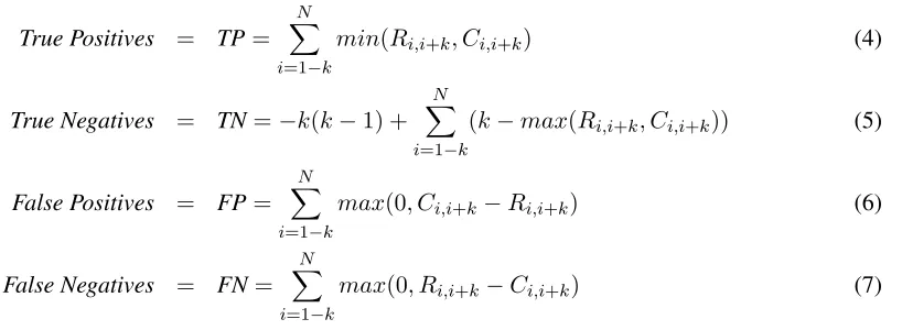
WinPR is derived from WindowDiff, but differs on one main point: WinPR evaluates boundary posi-tions, while WindowDiff evaluates regions (or win-dows). WinPR is a set of equations (4-7) (Figure 2) producing a confusion matrix. The confusion matrix allows for the distinction between false positive and negative errors, and can be used with Precision, Re-call, and F-measure. Furthermore, the window size may be changed to adjust near-miss sensitivity with-out affecting the the interpretation of the confusion matrix.

N is the number of content units and k repre-sents the window size. WinPR includes the Lam-prier (2008) correction, thus the sum is from1−k to N instead of 1 toN −k as with WindowDiff. min and max refer to the tradition computer sci-ence functions which select the minimal or maximal value from a set of two values. True negatives (5) start with a negative term, which removes the value of the phantom positions.

Each WinPR equation is a summation over all windows. To understand the intuition behind each equation, consider Figure 3. R and C represent the number of boundaries from the reference and com-puted segmentations, respectively, in the ith win-dow, up to a maximum ofk. The overlapping region represents the TPs. The difference is the error, while the sign of the difference indicates whether they are FPs or FNs. The WinPR equations select the differ-ence using themax function, forcing negative val-ues to 0. The remainder, up tok, represents the TNs.

k Ci

Ri

0 0 C R

TP

error

TN

Figure 3: WinPR within Window Counting Demostration

True Positives = TP=

N X

i=1−k

min(Ri,i+k, Ci,i+k) (4)

True Negatives = TN=−k(k−1) +

N X

i=1−k

(k−max(Ri,i+k, Ci,i+k)) (5)

False Positives = FP=

N X

i=1−k

max(0, Ci,i+k−Ri,i+k) (6)

False Negatives = FN=

N X

i=1−k

max(0, Ri,i+k−Ci,i+k) (7)

Figure 2: Equations for the WinPR confusion matrix

3 = (6/2). Each window contains 3 content units, thus we consider 4 potential boundary positions (the edges are inclusive).

A) Correct boundary

B) Missed boundary

C) Near boundary

D) Extra boundary

E) Extra boundaries

Figure 4: Example segmentations

Example A provides a baseline for comparison; B is a false negative (a missed boundary); C is a near miss; D is an extra boundary at the beginning of the sequence, providing an example of Lamprier’s criti-cism. E includes two errors near each other. Notice how the additional errors in E have have a very small impact on the WindowDiff value. Table 1 lists the number of correct and incorrect windows, and the WindowDiff value for each example.

Example Correct Incorrect WindowDiff

A 10 0 0

B 6 4 0.4

C 8 2 0.2

D 9 1 0.1

E 4 6 0.6

Table 1: WindowDiff values for examples A to E

WindowDiff should penalize an error k times, once for each window in which it appears, with the exception of near misses which have partial reward

and penalization. D is only penalized in one win-dow, because most of the other windows would be outside the sequence. E contains two errors, but they are not fully penalized because they appear in over-lapping windows. Furthermore, using a single met-ric does not indicate if the errors are false positives or false negatives. This information is important to the development of a segmentation algorithm.

If we apply WinPR to examples A-E, we get the results in Table 2. We will calculate precision and recall using the WinPR confusion matrix, shown un-der WinP and WinR respectively. You will note that we can easily see whether an error is a false posi-tive or a false negaposi-tive. As we would expect, false positives affect precision, and false negatives affect recall. Near misses manifest as equal parts false pos-itive and false negative. In example E, each error is counted, unlike WindowDiff.

Example TP TN FP FN WinP WinR

a 4 40 0 0 1 1.0

b 0 40 0 4 - 0

c 3 40 1 1 0.75 0.75

d 4 36 4 0 0.5 1.0

e 4 32 8 0 0.33 1.0

Table 2: WinPR values for examples A to E

fusion matrix (or normalized WinPR), as the con-fusion matrix divided by the window size. If near misses are not considered, this confusion matrix gives the exact count of boundary assignments.

What is not apparent in Table 2, is that WinPR is insensitive to window size, with the exception of near misses. Thus adjusting the window size can be used to adjust the tolerance or sensitivity to near misses. Large window sizes are more forgiving of near misses, smaller window size are more strict.

3.1 Near Misses and Window Size

WinPR does not provide any particular values in-dicating the number of near misses, their distance, or contribution to the evaluation. Because WinPR’s window size only affects near miss sensitivity, and not the positive/negative balance like in WindowD-iff, we can subtract two normalized confusion ma-trices using different window sizes. The difference between the confusion matrices gives the impact of near misses under different window sizes. Choosing a very strict window size (k= 1), and subtracting it from another window size would effectively provide the contribution of the near misses to the confusion matrix. In many circumstances, using several win-dow sizes may be desirable.

3.2 Variations in Segment Size: Validation by Simulation

We ran numerous tests on artificial segmentation data composed of 40 segments, with a mean segment length of 40 content units, and standard deviations varying from 10 to 120. All tests showed that a false positive or a false negative error is always penalized ktimes, as expected.

3.3 WinPR Applied to a Complete Segmentation

Using a reference segmentation of 40 segments, we derived two flawed segments: we added 20 extra boundaries to one, and removed 18 boundaries from the other. Both produced WindowDiff values of 0.22, while WinPR provided WinP = 0.66 and WinR = 1.0 for the addition of boundaries and WinP = 1.00 and WinR = 0.54 for the removal of bound-aries. WinPR highlights the differences in the na-ture of the two flawed segmentations, while WinDiff masks both the number and types of errors.

4 Conclusion

We presented a new evaluation method for segmen-tation, called WinPR because it produces a confu-sion matrix from which Preciconfu-sion and Recall can be derived. WinPR is easy to implement and provides more detail on the types of errors in a computed seg-mentation, as compared with the reference. Some of the major benefits of WinPR, as opposed to Win-dowDiff are presented below:

1. Distinct counting of false positives and false negatives, which helps in algorithm selection for downstream tasks and helps with analysis and optimization of an algorithm.

2. The confusion matrix is easier to interpret than a WindowDiff value.

3. WinPR counts errors from boundaries, not win-dows, thus close errors are not masked

4. Precision, and Recall are easier to understand than WindowDiff.

5. F-measure is effective when a single value is required for comparison.

6. WinPR incorporates Lamprier (2008) correc-tion.

7. Adjusting the window size can customize an evaluation’s tolerance of near misses

8. WinPR provides a method of detecting the im-pact of near misses on an evaluation

WinPR counts boundaries, not windows, which has analytical benefits, but WindowDiff’s counting of windows provides an evaluation of segmentation by region. Thus WindowDiff is more appropriate when an evaluator is less interested in the types and the number of errors and more interested in the per-centage of the sequence that is correct.

Acknowledgments

References

L Chen, YC Lai, and H Liao. 2008. Movie scene segmentation using background information. Pattern Recognition, Jan.

M Franz, J McCarley, and J Xu. 2007. User-oriented text segmentation evaluation measure. SIGIR ’07 Pro-ceedings of the 30th annual international ACM SIGIR conference on Research and development in informa-tion retrieval, Jan.

M Georgescul, A Clark, and S Armstrong. 2009. An analysis of quantitative aspects in the evaluation of the-matic segmentation algorithms. SigDIAL ’06 Proceed-ings of the 7th SIGdial Workshop on Discourse and Dialogue, Jan.

J Jancsary, J Matiasek, and H Trost. 2008. Revealing the structure of medical dictations with conditional ran-dom fields. EMNLP ’08 Proceedings of the Confer-ence on Empirical Methods in Natural Language Pro-cessing, Jan.

S Lamprier, T Amghar, and B Levrat. 2008. On evalu-ation methodologies for text segmentevalu-ation algorithms.

19th IEEE International Conference on Tools with Ar-tificial Intelligence - Vol.2, Jan.

I Malioutov and R Barzilay. 2006. Minimum cut model for spoken lecture segmentation. ACL-44 Proceedings of the 21st International Conference on Computational Linguistics and the 44th annual meeting of the Associ-ation for ComputAssoci-ational Linguistics, Jan.

I Malioutov, A Park, R Barzilay, and R Glass. 2007. Making sense of sound: Unsupervised topic segmen-tation over acoustic input. Proceeding of the Annual Meeting of the Association for Computation Linguis-tics 2007, Jan.

L Pevzner and M Hearst. 2002. A critique and improve-ment of an evaluation metric for text segimprove-mentation.

Computational Linguistics, Jan.