Hyper and structural Markov laws for graphical models

(1)

H

yper and

S

tructural

M

arkov

L

aws for

G

raphical

M

odels

Simon Byrne

Clare College and Statistical Laboratory,

Department of Pure Mathematics and Mathematical Statistics

This dissertation is submitted for the degree of Doctor of Philosophy

University of Cambridge

(2)

(3)

Declaration

This dissertation is the result of my own work and includes nothing which is the outcome of work done in collaboration except where specifically indi-cated in the text.

(4)

(5)

Acknowledgements

I would like to thank everyone who helped in the writing of this thesis, especially my supervisor Philip Dawid for the thoughtful discussions and advice over the past three years. I would also like to thank my colleagues in the Statistical Laboratory for their support and friendship. Finally I would like to thank my family, especially Rebecca, without whom I would never have been able to complete this work.

(6)

(7)

Summary

My thesis focuses on the parameterisation and estimation of graphical mod-els, based on the concept ofhyper and meta Markov properties. These state that the parameters should exhibit conditional independencies, similar to those on the sample space. When these properties are satisfied, parameter estima-tion may be performed locally, i.e. the estimators for certain subsets of the graph are determined entirely by the data corresponding to the subset.

Firstly, I discuss the applications of these properties to the analysis of case-control studies. It has long been established that the maximum like-lihood estimates for the odds-ratio may be found by logistic regression, in other words, the “incorrect” prospective model is equivalent to the correct retrospective model. I use a generalisation of the hyper Markov properties to identify necessary and sufficient conditions for the corresponding result in a Bayesian analysis, that is, the posterior distribution for the odds-ratio is the same under both the prospective and retrospective likelihoods. These conditions can be used to derive a parametric family of prior laws that may be used for such an analysis.

The second part focuses on the problem of inferring the structure of the underlying graph. I propose an extension of the meta and hyper Markov properties, which I term structural Markov properties, for both undirected decomposable graphs and directed acyclic graphs. Roughly speaking, it re-quires that the structure of distinct components of the graph are condition-ally independent given the existence of a separating component. This allows the analysis and comparison of multiple graphical structures, while being able to take advantage of the common conditional independence constraints. Moreover, I show that these properties characterise exponential families, which form conjugate priors under sampling from compatible Markov dis-tributions.

(8)

(9)

List of Figures

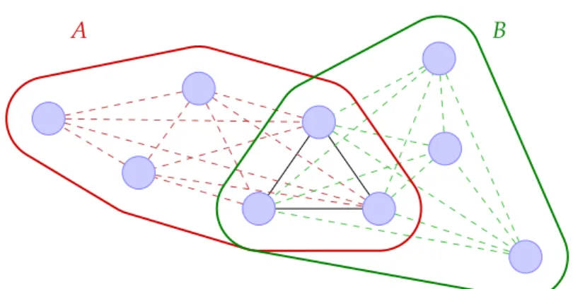
4.1 A representation of the structural Markov property for

undi-rected graphs. . . 44

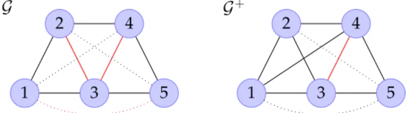
4.2 Neighbouring graphs on 5 vertices . . . 61

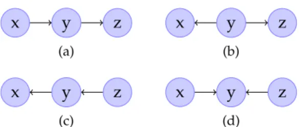
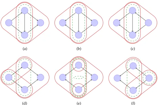
5.1 Four directed acyclic graphs with the same skeleton. . . 65

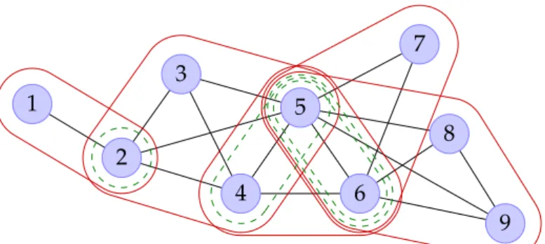
5.2 The d-cliques and d-separators of different graphs. . . 73

5.3 Three Markov equivalent graphs in which the same edge removal will result in a transition to a distinct Markov equivalence class. 79 A.1 The cliques of an undirected decomposable graph. . . 88

(12)

(13)

Part I

(14)

(15)

1

Graphical models and hyper Markov

properties

In this chapter, we introduce the necessary definitions and theorems for graphical models, in particular the role of conditional independence and the Markov properties of graphs.

The basis of this thesis involves the hyper Markov properties, introduced in a seminal paper by Dawid and Lauritzen (1993). We introduce the neces-sary terminology and results, but refer the reader to the original paper for more details. Finally, we review some of the notable subsequent develop-ments in hyper Markov theory.

1.1

Conditional independence

One of the most fundamental concepts of graphical models is the notion of conditional independence, which is used to describe the relationship be-tween random variables.

Definition 1.1.1 (Conditional independence). Let X,Y,Z be random vari-ables on a joint probability space (Ω,A,P). We say X is conditionally inde-pendent of Y given Z, written

X⊥⊥Y|Z [P],

if there exists a conditional probability measure for X given Y,Z under P that only depends on Z.

In circumstances where the distribution is implied, we may drop the[P]. If Zis trivial, then we havemarginal independenceand may writeX⊥⊥Y.

(16)

Under certain conditions, such as the lack of any functional relationship betweenX,Y,Z, we also have the following property:

C5 IfX⊥⊥Y|ZandX⊥⊥Z |Y, then X⊥⊥(Y,Z), though we will not utilise this property further.

1.2

Separoids and Graphical models

Graphical models encode a set of conditional independence properties in the structure of a graph. To facilitate later developments, we describe these conditional independence properties via the abstract separoid terminology of Dawid (2001), similar to thesemi-graphoid of Pearl and Paz (1987); Pearl (1988).

Definition 1.2.1. Let M be a set with elements of the formhA,B|Ciwhere A,B,C are subsets of a finite set V (that is, M is a ternary relation on V). ThenM is aseparoidif it satisfies the following properties:

S0 hA,B|Ai ∈M.

S1 IfhA,B|Ci ∈M, thenhB,A|Ci ∈M.

S2 IfhA,B|Ci ∈M andD⊆ A, thenhD,B|Ci ∈ M. S3 IfhA,B|Ci ∈M andD⊆ A, thenhA,B|C∪Di ∈ M.

(17)

1.2. Separoids and Graphical models Remark. Dawid (2001) actually defines a more general construction on a

semilattice, but the above characterisation is sufficient for our purposes. For each vertex v ∈ V, we define a random variable Xv on a sample space X_v. Furthermore, for any A ⊆ V we write the vector XA = (Xv)v∈V, the product spaceX_A =∏_v_∈_AXv, andX=XV andX =XV.

A joint distributionPforX isMarkovwith respect to a separoidM if:

hA,B|Ci ∈ M ⇒ XA⊥⊥XB |XC [P].

Specifically, we will focus on the separoids induced by graphs (see Ap-pendix A for the necessary graph terminology). We define theseparoid of an undirected graphG:

M(G) =

hA,B|Ci: AandBare separated byCinG . (1.1) The separoid of a directed acyclic graphG is the set:

M(G) =hA,B|Ci:AandBare separated byCin G_anm_(A_∪_B_∪_C) . (1.2) We say a distribution is Markov with respect to a graph, if it is Markov with respect to its separoid.

We note that properties S0–4 are constructive, that is, each specifies the existence of an element of the separoid. Therefore, by iteratively applying these properties to an arbitrary set N of such triples, we can generate all the elements of the smallest separoid containing N, which we the separoid closure of N, and denote by N. Furthermore, we say N is a spanning subset of N.

The link between the conditional independence properties C0–4, and the separoid properties S0–4, implies the following:

Lemma 1.2.1. Let N be a spanning subset of the separoid M, and P be a distribu-tion for X such that:

hA,B|Ci ∈ N ⇒ XA⊥⊥XB |XC [P]. then P is Markov with respect to M.

The separoid of an undirected decomposable graph can be generated by the decompositions of the graph:

(18)

Theorem 1.2.2(Dawid and Lauritzen 1993, Theorem 2.8). LetG be an undi-rected decomposable graph. Then the set:

hA,B|A∩Bi: (A,B)is a decomposition ofG

is a separoid spanning set forM(G).

Similarly, the separoid of a directed acyclic graph can be generated by the parent sets of individual vertices:

Theorem 1.2.3(Lauritzen, Dawid, et al. 1990, Propositions 4 and 5). LetG be a directed acyclic graph, with a well-ordering≺of the vertices. Then the sets:

{v}, ndG(v)| pa_G(v):v∈ V (1.3)

{v}, pr_≺(v)| pa_G(v)

:v∈ V (1.4)

are separoid spanning sets forM(G).

The sets (1.3) and (1.4) are known as thelocalandordered Markov proper-ties.

We note that for any separoid M, there is a natural projection onto a subsetU⊆ V:

MU =

hA,B|Ci ∈M : A,B,C⊆U

One interesting question is under what circumstances does this projection agree with the separoid of the induced subgraph,i.e.MU(G) =M(GU)? Theorem 1.2.4 (Asmussen and Edwards 1983, Corollary 2.5). Let G be an undirected graph. ThenM_U(G) =M(GU)if and only ifG is collapsible onto U.

For the directed case, there is no known characterisation of such sets, however there is the following sufficient condition:

Theorem 1.2.5. Let G be a directed acyclic graph. If U is an ancestral set, then

M_U(G) =M(GU).

Another useful property is that the separoids of edge subgraphs are in fact larger:

Theorem 1.2.6. Let G,G0 _{be either undirected or directed acyclic graphs on V.}

Then:

E(G)⊆ E(G0) ⇒ M(G)⊇ M(G0).

In other words, ifP is Markov with respect toG, and G is an edge sub-graph ofG0, thenPmust also be Markov with respect toG0.

(19)

1.3. Hyper Markov properties

1.3

Hyper Markov properties

We define amodel to be a family of probability distributionsΘ over a com-mon measurable space. Specifically, we will focus on the case where Θ ⊆

P(G), the set of distributions that are Markov with respect to a graphG. For any θ ∈ Θ and A ⊆ V, define θA to be the marginal distribution of XA underθ. Moreover, for A,B ⊆ V, we define θ_A_|_B to be the family of

conditional distributions of (XA|XB = xb)xb. If we use φ ' ψ to denote

the existence of a bijective function between φ andψ, we note that for any

A⊆V, (Dawid and Lauritzen 1993, Lemma 3.1)

θ '(θA,θ_V\A|A).

A law £ is a probability distribution of a random distribution ˜θ taking

values in Θ. As we primarily focus on Bayesian methodology, we will use laws to describe the prior and posterior distributions for statistical models, though Dawid and Lauritzen (1993) also used laws in the context of sam-pling distributions of estimators.

A law£(θ˜) for an undirected graph G is (weak) hyper Markov if for any

decomposition(A,B)ofG: ˜

θA⊥⊥θ˜B |θ˜A∩B [£] (1.5) We note that both weak hyper Markov properties may be characterised in terms of their separoids:

Theorem 1.3.1. A £(θ˜)is weak hyper Markov with respect to an undirected

de-composable or directed acyclic graphG if and only if: ˜

θA∪C⊥⊥θ˜B∪C |θ˜C [£] (1.6) for allhA,B|Ci ∈ M(G).

Proof. By Theorems 1.2.2 and 1.2.3, we simply need to show that there are analogous properties to properties S0–4: that is, for every A,B,C,D ⊆

V:

H0 θ˜A∪A⊥⊥θ˜B∪A |θ˜A∪A.

(20)

H2 If ˜θA∪C⊥⊥θ˜B∪C|θ˜C andD⊆ A, then ˜θD∪C⊥⊥θ˜B∪C |θ˜C.

H3 If ˜θA∪C⊥⊥θ˜B∪C|θ˜C andD⊆ A, then ˜θA∪C∪D⊥⊥θ˜B∪C∪D |θ˜C∪D. H4 If ˜θA∪C⊥⊥θ˜B∪C | θ˜C and ˜θA∪B∪C⊥⊥θ˜D∪B∪C | θ˜B∪C, then ˜θA∪C⊥⊥

˜

θD∪B∪C |θ˜C.

H0–2 and H4 follow immediately by the properties of conditional indepen-dence C0–4. To show H3, we note thatθC∪D ' (θC,θ_D|C), and hence:

˜

θA∪C∪D⊥⊥θ˜B∪C⊥⊥θ˜D∪C

Furthermore, asXD⊥⊥XB|XC, then we haveθB∪C∪D ' (θB∪C,θ_D|C). As a consequence of this and Theorem 1.2.6:

Corollary 1.3.2. If £ is hyper Markov with respect toG, andE(G)⊆ E(G0₎_{, then}

£ is hyper Markov with respect toG0.

However, for much of the work in this thesis, we will utilise the stronger property:

Definition 1.3.1 (Strong hyper Markov property). A law £(θ˜) is strong

hy-per Markovwith respect to an undirected decomposable graph G if for any decomposition(A,B)of G:

˜

θ_B|A⊥⊥θ˜A [£]. (1.7) A law £(θ˜) isstrong directed hyper Markov with respect to a directed acyclic

graphG if for every vertexv ∈V: ˜

θ_v|pa(v)⊥⊥θ˜nd(v) [£]. (1.8) Interestingly, there is no corresponding property to Corollary 1.3.2: if£is strong hyper Markov with respect toG, it need not be strong hyper Markov with respect toG0 _{⊇ G} _{(though it will still be weak hyper Markov), as we}

will see in Example 1.6.1 below.

One of the key benefits of strong hyper Markov laws is that when used as prior distributions in a Bayesian analysis, the posterior updating may be done locally:

(21)

1.4. Constructing hyper Markov laws Theorem 1.3.3 (Dawid and Lauritzen 1993, Corollary 5.5). If the prior law

£(θ˜)is strong hyper Markov, and x is a completely observed realisation of X, then

the posterior £(θ˜|X= x)is strong hyper Markov, and for any clique C

£(θ˜C|X =x) =£(θ˜C|XC = xc)

1.4

Constructing hyper Markov laws

One of the convenient aspects of conditional independence is that it allows us to define distributions in a piecewise manner.

Theorem 1.4.1 (Dawid and Lauritzen 1993, Lemma 2.5). Let Q be a distribu-tion for XA and R for XB, such that QA∩B = RA∩B, then there exists a unique distribution P for XA∪B such that:

(i) PA= Q, (ii) PB =R, and

(iii) XA⊥⊥XB |XA∩B [P].

Importantly, we can apply the same procedure to laws:

Theorem 1.4.2(Dawid and Lauritzen 1993, Lemma 3.3). LetM(θ˜A)be a law for XA, andN(θ˜B)be a law for XB such thatMA∩B =NA∩B. Then there exists a unique law £(θ˜A∪B)such that:

(i) £A =M, (ii) £B =N,

(iii) θ˜A⊥⊥θ˜B |θ˜A∩B [£], and

(iv) XA⊥⊥XB |XA∩B [θ˜],almost surely under £.

Dawid and Lauritzen (1993) termQ andR to beconsistent, and P to be theirMarkov combination, denoted by the operationP= Q?R. Likewise,M

andN are hyper consistent, and£is theirhyper Markov combination, denoted by£=M N.

Both of these operations are products in a category-theoretic sense: they are defined uniquely by their marginal projections. This concept of a condi-tional productwas explored by Dawid and Studený (1999), who explored its axioms and how they relate to those of conditional independence.

(22)

We can use these to construct Markov distributions and hyper Markov laws on undirected decomposable graphs by specifying marginal distribu-tions and laws on cliques, and sequentially applying the above operadistribu-tions. Specifically, if(P(C))_C_∈_cl₍_G₎are a set of pairwise consistent distributions, then the distribution:

?

C∈cl(G)

P(C) (1.9)

is Markov with respect toG. Likewise, if

£(C)₍_θ˜_C₎

C∈cl(G) are a set of pair-wise hyper consistent laws, the law:

C∈cl(G)

£(C) (1.10)

will be hyper Markov with respect toG.

How does one obtain a set of consistent distributions or hyper consistent laws? One method is to simply take an arbitrary joint distribution or law for XV, and take the marginal distributions or laws on the cliques; these will by necessity be (hyper) consistent

Finally, as much of our focus will be on strong hyper Markov laws, we would like to know under what conditions the resultant law will be strong hyper Markov:

Theorem 1.4.3(Dawid and Lauritzen 1993, Proposition 3.16). A weak hyper Markov law £(θ˜)is strong hyper Markov if and only if the marginal law £(θ˜C)for each clique C is strong hyper Markov.

In other words, (1.10) is strong hyper Markov if and only if each £(C) is strong hyper Markov with respect to the complete graph onC.

1.5

Variation independence and meta Markov

properties

We can obtain similar properties by replacing the probabilistic independence with variation independence:

Definition 1.5.1. Letφ,ψandωbe functions on a common domainD. Then

we define theconditional range of φgivenω to be the image underφ of the

fibre ofω:

(23)

1.6. Gaussian graphical models and Hyper inverse Wishart laws Furthermore, we define φto be conditionally variation independent of ψgiven

ω, written:

φ ‡ ψ|ω [D]

if the conditional range of φ given (ψ,ω) is constant in ψ. That is, for all

v∈ψ(D),w∈ ω(D):

φ(ψ,ω)−1(v,w)=φω−1(w).

We note that the relation (· ‡ · | ·) satisfies the same properties C0–4, and hence

If we replace the probabilistic independence of the hyper Markov prop-erties with variation independence, we obtainmeta Markovproperties: Definition 1.5.2. LetG be an undirected graph. Then a modelΘ⊆P(Θ)is (weak) meta Markovif:

θA ‡ θB |θA∩B [Θ]

for all decompositions(A,B)ofG. Likewise,Θisstrong meta Markovif:

θ_B_|_A ‡ θ_A [Θ].

for all decompositions(A,B)ofG.

As we shall see in the next chapter, the variation independence has an important role in the properties of the maximum likelihood estimators, par-ticularly when the data are obtained from different sampling regimes. More-over, the support of weak/strong hyper Markov laws will be weak/strong meta Markov. As such, the lack of a meta Markov model will preclude the existence of a corresponding hyper Markov law.

1.6

Gaussian graphical models and Hyper inverse

Wishart laws

One of the most common graphical models is the multivariate Gaussian graphical model, also called the covariance selection model (Dempster 1972; Wermuth 1976a). LetX= _∏_v_∈_VXv, then:

(24)

In particular,θ is Markov with respect to an undirected graphG if:

{u,v}∈ E/ (G) ⇒ Λ_uv =0 (1.11) whereΛ=Σ−1_{is the}_{precision matrix}_.

For any disjoint A,B ⊆ V, the marginal and conditional distributions are:

θA'ΣAA and θ_B|A'(ΓB|A,ΣB|A)

The conjugate prior law for the complete model is theinverse Wishart law, £(θ˜) = I W(δ;Φ), using the notation of Dawid (1981). In particular, this

law is strong hyper Markov on the complete graph, since for any disjoint A,B⊆V: ˜ θA⊥⊥θ˜_B_|_A [£] where: £(Σ˜_AA) =I W(δ;ΦAA) £(Σ˜_B_|_A) =I W(δ+|A|;Φ_B|A) £(Γ˜_B_|_A|_Σ˜_B_|_A) =Φ_BAΦ−_AA1 +N_B_×_A(Σ˜_B_|_A,Φ−_AA1)

The hyper Markov law constructed by the hyper Markov combination on the cliques (1.10) is termed thehyper inverse Wishart. Moreover, since any clique marginal law is strong hyper Markov with respect to the complete graph, then by Theorem 1.4.3, the hyper inverse Wishart is also strong hyper Markov.

Interestingly, this property is generally unique to the inverse Wishart law:

Theorem 1.6.1 (Geiger and Heckerman 2002, Theorem 7). LetG be the com-plete graph on 3 or more vertices. Then the law for the Gaussian graphical model onG is strong hyper Markov if and only if it is an inverse Wishart law.

However, if there are only two vertices in the clique, then the family of strong hyper Markov laws is slightly more general:

(25)

1.6. Gaussian graphical models and Hyper inverse Wishart laws Theorem 1.6.2(Geiger and Heckerman 2002, Theorem 12). LetG be the

com-plete graph on 2 vertices. Then the law for the Gaussian graphical model on G is strong hyper Markov if and only if it has a density on the precision space of the form:

h(Λ₁₂)|Λ|−δ/2−2_exp_{−1

2tr(ΦΛ)},

for some arbitrary function h.

These results, when combined with Theorem 1.4.3, severely limit the choice of possible strong hyper Markov laws for the Gaussian model.

For example, Letac and Massam (2007) and Rajaratnam, Massam, and Carvalho (2008) define a more general family of the hyper inverse Wishart law, which they term a “Type II Wishart”. This law obeys the directed strong hyper Markov law (for a given perfect ordering of cliques), but due to the above results, will not generally be strong hyper Markov with respect to an undirected graph.

Also of interest is the corresponding law on the precision matrix:

Theorem 1.6.3 (Roverato 2000, Equation 13). If £(Σ˜) =H I W_G(δ;Φ), then

corresponding law forΛ˜ = Σ˜−1has a density proportional to:

|Λ|(δ−2)/2_exp

−1

2tr(ΦΛ)

forΛ∈ P+

G(0), the set of positive definite matrices satisfying(1.11).

In particular, we note that this is exactly proportional to the density of the Wishart lawW(δ+p−1;Φ−1), albeit concentrated onP_G+₍₀₎. This means

that the hyper inverse Wishart law may be obtained from the inverse Wishart by appropriately conditioning on the precision matrix:

Corollary 1.6.4. If £(Σ˜) =I W(δ;Φ), then:

£ Σ˜|_Λ˜_uv=0,{u,v}∈ E/ (G)

=H I W_G(δ;Φ)

Corollary 1.6.4 suggests a way that we might extend the definition of the hyper inverse Wishart law to non-decomposable graphs. For example, with the graph:

1 2 3 4

(26)

we can define the hyper inverse Wishart law as the conditional law given

λ13 = λ24 = 0. This approach was investigated by Roverato (2002) and

Atay-Kayis and Massam (2005). However, we note that the corresponding weak hyper Markov propertyM(G), namely:

˜

θ{1,2,3}⊥⊥θ˜{1,3,4} |θ˜{1,3} and θ˜{1,2,4}⊥⊥θ˜{2,3,4} |θ˜{2,4},

does not hold. Interestingly, there are still some strong hyper Markov-type properties, for example ifCis a clique, then:

˜

θ_V|C⊥⊥θ˜C.

Furthermore, the normalisation constant of such a density generally does not have a closed-form solution.

Finally, we note that unlike the Markov and weak hyper Markov prop-erties, if a graph is strong hyper Markov with respect to G, it need not be strong hyper Markov with respect toG0_{, where}_E₍_G0₎_{⊇ E}₍_G₎_:

Example 1.6.1. Suppose we have the Gaussian model on 3 vertices, that is Markov with respect to the graph:

1 2 3

Then we can parameterise this model by the incomplete covariance matrix: Σ∗ ₌    σ11 σ12 ∗ σ12 σ22 σ23 ∗ σ23 σ33   .

In the completion of this matrix, the missing element∗=σ13 =σ12σ23/σ22.

We now investigate the partition of the parameters into (θ_{_1,3_},θ₂_|{_1,3_}).

Note that: |σ12| ≤ √ σ11σ22 and |σ23| ≤ √ σ22σ33 ⇒ |σ13| ≤ √ σ11σ33

and so θ_{_1,3_} ' Σ_{_1,3_} may be any positive-semidefinite 2×2 matrix.

Fur-thermore, the regression coefficients of 2 on{1, 3}will be: Γ2|{1,3} = " σ₁₂ σ23 #>" σ₁₁ σ₁₂σ23/σ22 σ12σ23/σ22 σ33 #−1 = 1 σ11σ₂₂2σ33−σ₁₂2σ₂₃2 σ22σ12(σ22σ33−σ₂₃2 ),σ22σ23(σ11σ22−σ₁₂2)

(27)

1.7. Contingency tables and Hyper Dirichlet laws • If σ13 = 0, then Γ2|{1,3} = (σ12/σ11,σ23/σ33). However this would also

imply that eitherσ12orσ23 =0, and henceΓ2|{1,3} can only take values

on the axesR× {0} ∪ {0} ×_R.

• Ifσ13> 0, then it follows thatσ12σ23 > 0, and by examining the terms

of the above expression, it follows that Γ₂|{1,3} can only take values in

the quadrants(R>0)2∪(R<0)2

• If σ13 <0, then σ12σ23 < 0, and by similar inspection,Γ2|{1,3} can only

take values in the quadrants (R>0×R<0)∪(R<0×R>0).

As the range of Γ₂_|{_1,3_} depends on the value of σ13, then θ₂_|{_1,3_} and θ_{_1,3_}

are not variation independent. Therefore the model cannot be strong meta Markov on the complete graph, nor can any law with full support, such as the hyper inverse Wishart, be strong hyper Markov on this graph.

1.7

Contingency tables and Hyper Dirichlet laws

The other common graphical model is the contingency table. If the variable Xis discrete sample space X_v is finite, then each cell x = (xv)v∈V ∈ X will have probability θ(x).

Such models are usually parameterised in log-linear form (see, for exam-ple, Darroch, Lauritzen, and Speed 1980), but for our purposes it is easier to work with the clique-marginal distributions. Specifically, for any clique C, we let θ(xC)be the marginal probability of any cellxc∈ XC.

Then the probability of any cellx ∈ X is:

θ(x) =

∏

C∈cl(G) θ(xC)

∏

S∈sep(G) θ(xS)νG(S)

where νG(S)denotes the multiplicity of a separatorS.

The standard conjugate prior on the complete graph is the Dirichlet law £(θ˜) = D(α), where the parameter α : X → R>0. This is a strong hyper

Markov law, and:

£(θ˜A) =D(αA) £ θ˜_B|A(· |xA) =D αA∪B(·,xA) where αA(xA) =∑x0_:_x0 A=xAα(x)

(28)

The hyper Markov combination of a set of consistent Dirichlet laws is thehyper Dirichlet law, which by Theorem 1.4.3, must also be strong hyper Markov.

Interestingly, this is not the only strong hyper Markov law. Consider a 2×2 table, with θxy = θ(x,y). Geiger and Heckerman (1997, equation 10)

note that a law is strong hyper Markov if and only if it has a density of the form: h θ00θ11 θ01θ10 θ₀₀α00−1θα₀₁01−1θα₁₀10−1θ₁₁α11−1 (1.12)

for some functionh. In the case wherehis constant, this is simply a Dirichlet distribution.

We can the extend sufficient condition to larger tables:

Theorem 1.7.1. If a law £(θ˜)for a 2-way contingency table X×Y on X × Yhas

density: h θxyθx∗_y∗ θxy∗_θ_x∗_y x6=x∗_,_y₆_=y∗ !

∏

x,y θαxyxy−1, (1.13) then it is strong hyper Markov.

Proof. The Jacobian determinant of the transformationθxy 7→(θ+y,θ_x_|_y)is:

dθxy d(θ+y,θ_x|y) =

∏

y θ_+y|X |−1

(see, for example, Heckerman, Geiger, and Chickering 1995, Theorem 10), which gives the joint density for(θ+y,θ_x_|_y):

∏

y θα_+y+y−1h   " θ_x|yθx∗_|_y∗ θ_x|y∗θ_x∗_|_y # x6=x∗_,_y₆_=y∗  

∏

x,y θ_xαxy_|_y−1 (1.14)

which factorises into a term involving onlyθ+yterms, and another involving only θ_x|y terms. Therefore ˜θY⊥⊥θ˜_X|Y. By symmetry, the same argument holds in the other direction.

It is unclear if the converse is true: the corresponding result in (1.12) re-lies on results from functional equations, and it is unclear if these arguments can be extended directly to higher dimensions.

The form of the density in Theorem 1.7.1 assumes the law has full sup-port. However, as we shall demonstrate in the next chapter, we can obtain

(29)

1.7. Contingency tables and Hyper Dirichlet laws strong hyper Markov laws on submanifolds by conditioning on the

odds-ratio parameter. Furthermore, the form of the density in (1.14) gives the following:

Corollary 1.7.2. If a law £(θ˜)satisfies the conditions of Theorem 1.7.1, the marginal

laws are:

£(θ˜X) =D(αX) and £(θ˜X) =D(αY).

Example 1.7.1. One way to construct such a law is through a mixture of Dirichlet laws£(θ˜|α˜) =D(α˜), where the law for the mixing parameter£(α˜)

has constant marginals:

£(α˜x+ =ax+) =1 and £(α˜+y =a+y) =1. By the properties of the Dirichlet law, we have:

˜

θY⊥⊥θ˜_X_|_Y |α˜ and θ˜X⊥⊥θ˜_Y_|_X|α˜ [£].

Furthermore, the constant marginal laws imply that ˜θY⊥⊥α˜ and ˜θX⊥⊥α˜, and

so:

˜

θY⊥⊥(θ˜_X|Y, ˜α) and θ˜X⊥⊥(θ˜_Y|X, ˜α) [£].

Therefore£(θ˜)is strong hyper Markov. Now defineaxy = ax+a+y/a++, and: ˜

ηxy = α˜xy−axy, x6= x∗,y6=y∗ Furthermore, note that:

˜ αx∗_y =_α˜_+y−

∑

x6=x∗ ˜ αxy = ax∗_y−

∑

x6=x∗ ˜ ηxy, y6=y∗ ˜ αxy∗ =_α˜_x+−

∑

y6=y∗ ˜ αxy =axy∗−

∑

y6=y∗ ˜ ηxy, x 6= x∗ ˜ αx∗_y∗ =_α˜_+y∗−

∑

x6=x∗ ˜ αxy∗ = a_x∗_y∗+

∑

x6=x∗_,_y₆_=y_∗ ˜ ηxy.

Therefore, ˜η completely characterises the mixing vector. £(θ˜) has a density

of the form: π(θ) =E_£(_α_˜)[π(θ|α˜)] =Eα˜ " 1 B(α˜)

∏

_x_,_yθ ˜ αxy−1 xy # . This may be re-expressed as:

π(θ) =

∏

x,y θaxyxy−1E£(α˜, ˜η) " 1 B(α˜)_x₆_=x

∏

∗_,_y₆_=y∗ θxyθx∗_y∗ θxy∗_θ_x∗_y η˜xy# (1.15) which is of the same form as the density in Theorem 1.7.1.

(30)

Unfortunately, for most functions h, the normalisation constant of the density (1.13) will usually not have an analytic form. Even for Example 1.7.1, the occurrence of the beta function inside the integral in (1.15) will usually mean that the precise form of the density is intractable, other than for finite mixtures.

Theorem 1.7.1 may be extended to higher-order tables, but the arbitrary functionhis limited to the highest order interaction term:

Theorem 1.7.3. If a law £(θ˜)for an n-way contingency table X = ∏_v∈VXv has density of the form:

h   "

∏

B⊆V θ(x∗_B,x_V_\_B)(−1) |V\B| # x:xv6=x∗ v  

∏

x θ(x)α(x)−1 (1.16)

then it is strong hyper Markov.

Proof. For any ∅ ⊂ A ⊂ V, let Ac = V\A, and note that the first product term in (1.16) may be written as:

∏

C⊆AD

∏

⊆Ac

θ(x_C∗,x_A\C,x∗D,xAc_\_D)(−1)

|A\C|+|Ac\D|

. This may be rewritten as:

∏

C⊆A " θ(x_C∗,x_A_\_C,x∗_AC)

∏

D⊂Ac θ(x∗_C,x_A_\_C,x∗_D,x_Ac_\_D)(−1) |Ac\D| #(−1)|A\C| (1.17) Recall that any finite, non-empty set has an equal number of even and odd size subsets, therefore:

∑

D⊂Ac

(−1)|Ac\D| = −1, and so (1.17) may be expressed as:

∏

C⊆A  

∏

D⊂Ac θ(x_C∗,x_A\C,x∗D,xAc_\_D) θ(x∗_C,x_A_\_C,x∗_Ac) !(−1)|Ac\D|  (−1)|A\C|

By the same argument overC, we obtain:

∏

C⊂AD

∏

⊂Ac θ(x∗_C,x_A_\_C,x∗_D,x_Ac_\_D) θ(x∗_C,x_A\C,x∗Ac) θ(x∗_A,x∗_Ac) θ(x∗_A,x∗_D,x_Ac_\_D) !(−1)|A\C|+|Ac\D|

Note that the term inside the parenthesis is of the same form as the fraction in (1.13), and hence satisfies the conditions of Theorem 1.7.1 (with x = xA andy= xAc), and therefore ˜θA⊥⊥θ˜_V|A.

(31)

1.8. Notes and other developments Furthermore, this link to Theorem 1.7.1 means that we have a similar

result to Corollary 1.7.2:

Corollary 1.7.4. If a law £(θ˜) satisifies Theorem 1.7.3, then for any A ⊂ V, the

marginal law £(θ˜A) =D(αA).

1.8

Notes and other developments

The Dirichlet process (Ferguson 1973) is a law on an arbitrary measurable space, and may be regarded as an infinite-dimensional extension of the Dirichlet law. It has many interesting properties, notably that the result-ing probability measure is almost surely discrete.

Asci, Nappo, and Piccioni (2006) and Heinz (2009) independently de-velop the hyper Dirichlet process, defined as a hyper Markov combination of consistent Dirichlet processes on the cliques. Unlike the hyper Dirichlet law however, it is generally not strong hyper Markov. In fact, under quite general conditions—such as the base measures being continuous and the graph G being connected—it will simply be a Dirichlet process whose base measure is the Markov combination of the clique base measures, in other words:

C∈cl(G) DP(µC,A) =DP

?

C∈cl(G) µC,A ! .

This is due to the inherent discrete nature of the Dirichlet process. If θ is

drawn from a Dirichlet processDP(µ,A)on some product spaceX × Y ×

Z, then it will (almost surely) have a representation of the form:

θ =

∑

i

aiδ_(xi_,_yi_,_zi)

where the coordinates (xi,yi,zi)are drawn i.i.d. from µ, and δ is the Dirac

measure. Ifµis continuous, then the probability of there being two distinct

coordinates(xi,yi,zi)and(xj,yj,zi)such thatyi = yj will be zero. Therefore, if a triple(X,Y,Z)is drawn fromθ, thenθ(X= xi,Z=zi|Y= yi) =1, and hence, somewhat trivially, we have the Markov property:

X⊥⊥Z|Y [θ].

Finally, we note that although the strong hyper Markov property is very restrictive, such laws can form useful building blocks in constructing more

(32)

general laws. One common approach is to specify the law in an hierarchical manner, by specifying a family of strong hyper Markov laws as well as a mixing distribution over this family (often called ahyperprior).

We note that the resultant marginal law will usually not be strong, or even weak, hyper Markov (Example 1.7.1 being an exception). Nevertheless, such an approach can still be advantageous, as the conditional independence properties may still be exploited for computational purposes.

For example, suppose that £(θ˜|α˜) is a family of hyper Dirichlet laws,

and£(α˜)describes the mixing law. Then by exploiting the conditional hyper Markovity and the fact that:

X⊥⊥α˜ |θ˜ [£]

we could construct a Markov chain Monte Carlo algorithm to obtain a sam-ple from the posterior by alternating the following steps:

a) For each cliqueCi, independently sample:

θ_C(n+1)

i|Si ∼£( ˜

θ_Ci|Si|α(n),XC = xc),

whereSi is theith separator in a perfect orderingC1, . . . ,Ck. b) Sample:

α(n+1) ∼£(α˜ |θ(n+1)).

In this case, step (a) may be performed in parallel on up to k processors. This is particularly useful in the case where the evaluation of the likelihood function is computationally intensive. Furthermore, each processor would only require the dataXCi of the corresponding clique.

(33)

2

Logistic regression and case-control

studies

An interesting application of the meta Markov and hyper Markov properties arises in analysis of case-control studies.

If one wishes to determine particular risk factors for a disease (or any other binary outcome), there are two basic approaches:

Prospective or cohort study Select subjects from the population based on their risk factors, and observe them at the end of a fixed time period to determine if the disease arises.

Case-control or retrospective study Choose a random sample of subjects from the population with the disease (cases), and another sample from the population without (controls). Compare the relative frequencies of the risk factors in the two samples.

Let Ybe the response variable taking values in{0, 1}, corresponding to the absence or presence of disease, respectively (the following results may be extended to the multinomial case, but for sake of simplicity we only pursue the binomial). LetXbe the covariates (risk factors) taking values inX ⊆Rk_. In a prospective study we are observing the conditional distribution of Y givenX, and so under a proportional odds assumption, we obtain the model for logistic regression:

p(y|x,α,β) = e

y(α+β>x)

1+eα+β>x, α∈R,β∈R

k_. _(2.1)

On the other hand, a case-control study will result in observations from the conditional distribution of X givenY. In this case, specifying a proba-bilistic model becomes much more difficult, particularly if X is infinite.

Despite these difficulties, case-control studies are often desirable—or in some cases unavoidable—particularly where the disease is relatively rare or

(34)

the time until diagnosis may be particularly long, as the costs of obtaining a sufficient sample size for a prospective study are likely to be prohibitive.

The classic result of Prentice and Pyke (1979) showed that the maximum likelihood estimate and asymptotic covariance for the log-odds ratio param-eter βcould simply be found by logistic regression. In other words, we can

use the prospective model to analyse data gathered retrospectively. This particular result has been widely applied in epidemiology and other areas.

In this chapter, we identify the analogous result for the Bayesian case: that is, the conditions under which the posterior distribution for βmay be

computed using the prospective likelihood instead of the retrospective. The simplest model of a single binary covariate has been well explored in literature: Zelen and Parker (1986), Nurminen and Mutanen (1987), Marshall (1988) and Ashby, Hutton, and McGee (1993) have all characterised such an analysis, which consists of computing the posterior log odds ratio of a 2×2 contingency table under a Dirichlet prior.

In the case where the covariates are categorical, that is whereX is finite, Seaman and Richardson (2004) identified a class of improper priors that satisfy the desired properties. This class was further expanded by Staicu (2010).

We show that the basis of this prospective–retrospective symmetry is due to “independence” of the parameters: the original result of Prentice and Pyke (1979) can be explained through the variation independence of the parameter space, and that the corresponding Bayesian result will occur when the prior law exhibits analogous probabilistic independence. Further-more, we arrive at the same class of prior laws as Staicu (2010) via a different route, and demonstrate how they might be extended to stratified designs.

However it should be noted that this is not the only approach for Bayesian analysis of case-control data. With the advent of computational tools such as MCMC, the retrospective likelihood need not present such an obsta-cle. Indeed this path has been well followed in the literature, as reviewed in Mukherjee, Sinha, and Ghosh (2005). For example, Müller and Roeder (1997), Seaman and Richardson (2001) and Gustafson, Le, and Vallée (2002) have pursued this approach. In particular, Gustafson, Le, and Vallée (2002) note that in general the prospective posterior can serve as a useful approxi-mation to the retrospective posterior, and use this as the basis of an impor-tance sampling scheme.

(35)

2.1. Notation and definitions

2.1

Notation and definitions

Throughout the chapter, (X,Y) will be a single joint observation from the specified model, and (X(n),Y(n)) to be a sequence of n such independent observations. pwill be the density of the model (with respect to the appro-priate measure), with variables indicating the context.

Lemma 2.1.1. For the above logistic model, we have:

θ_Y|X'(α,β) and θX|Y ' (θX|Y=0,β) (2.2)

Proof. The first is determined by (2.1), and the second by Bayes theorem: dθ_X_|_Y=₁ dθ_X|Y=0 (x) = θY|X=x(1) θ_Y|X=x(0) θY(0) θY(1) ∝ eβ>x

2.2

Maximum likelihood estimators

Prentice and Pyke (1979) showed that the maximum likelihood odds-ratios obtained from a case-control study have the same properties as those arising from a prospective study, and hence may be found via logistic regression. This can be elegantly demonstrated by the strong meta Markov property. Lemma 2.2.1. LetΘXbe the family of all probability distributions overX, and let ΘY|X be the family of conditional distributions with densities of the form in(2.1). Then the corresponding family of joint distributionsΘis strong meta Markov, that is:

θX ‡ (α,β) and θY ‡ (θ_X|Y=0,β)

Proof. These properties are essentially a reformulation of Müller and Roeder (1997, Lemmas 1 and 2). By definitionθX ‡ θ_Y|X. It remains to show variation independence in the opposite direction.

For anyθXandθ_Y_|_X, the joint distribution θhas a density of the form:

p(x,y|θ) = e

y(α+β>x)

1+eα+β>xp(x|θX) (2.3)

Therefore the marginal distributionθY is Bernoulli, with parameterγtaking

values on the interval(0, 1), where:

γ= p(y=1|θ_Y) =

Z

X

eα+β>x

(36)

θ_Y0_|_X' (α0,β)∈Θ_Y_|_X such that α0 = α−log γ

1−γ

+log γ

0

1−γ0, (2.6)

andθ0_X has density:

p(x|θ0_X) = (1−γ

0₎₍₁₊_eα0+β>x₎

(1−γ)(1+eα+β>x)

p(x|θX)

By the definition ofγin (2.4), it can be shown that this integrates to 1, hence θ0_X ∈ ΘX. Furthermore, by matching terms in (2.5), then θ_X|Y = θ0X|Y. Since

θ_Y0 'γ0 may be chosen arbitrarily, it follows thatθY ‡ θ_Y|X.

The logistic model has other variation independence properties: Corollary 2.2.2. Under the logistic model of Lemma 2.2.1, then:

(θX,θY) ‡ β

Proof. We haveθX ‡ (α,β), and for anyθY, we can chooseα0 as in (2.6).

Theorem 2.2.3. Suppose we have a joint model as in Lemma 2.2.1. Then the profile likelihood function for the odds ratioβ is the same for both the retrospective model

ΘX|Y and the prospective modelΘY|X, up to proportionality.

Proof. This proof follows a similar argument as Dawid and Lauritzen (1993, Lemma 4.10). The joint density for the modelθ may be written as:

p(x,y|θ) =p(x|θX)p(y|x,α,β) = p(y|θY)p(x|y,θ_X|Y=0,β) (2.7)

Therefore the profile likelihood for the joint model may be written in terms of the prospective model:

Ljointp (β) =max

α,θX

p(x|θX)p(y|x,θ_Y|X) (2.8) By Lemma 2.2.1, the variation independence α and θX the factors of (2.8) may be profiled separately, and hence:

Ljointp (β)∝max

α p

(37)

2.3. Bayesian analysis of case-control studies where Lprop denotes the profile likelihood of the prospective model. The

same argument applies to the retrospective profile likelihoodLret_p (β):

Ljointp (β)∝ max

θX|Y=0

p(x|y,θ_X_|_Y=₀,β) =Lret_p (β)

From this we obtain the result of Prentice and Pyke (1979):

Corollary 2.2.4. For data observed in a case control study, the maximum likelihood estimate of the log odds parameterβˆand its asymptotic covariance may be computed

as if the data were observed prospectively, that is, using logistic regression.

Proof. The maximum likelihood estimator is a function of the profile likeli-hood, as is the asymptotic covariance (see Patefield 1985).

The same argument may be extended trivially to any penalised logistic regression estimator of the form:

arg max

α,β

logp(y|x,α,β) +φ(β).

Examples of such estimators include ridge regression, where φ(β) ∝ kβk2,

and lasso, where φ(β) ∝ kβk1. Such methods have proven successful in

genome-wide association studies (GWAS), which involve case-control data with extremely high-dimensional covariates (Park and Hastie 2008; Wu et al. 2009).

2.3

Bayesian analysis of case-control studies

We now investigate how these results correspond to a Bayesian analysis. We will use π to denote the density of the prior law, and πpro and πret to

denote the densities of the posterior laws £pro and £ret under prospective and retrospective likelihoods, respectively:

πpro(α,β|x(n),y(n))∝π(α,β)p(y(n)|x(n),α,β)

Furthermore, we will use ¯p to denote the density of the marginal model, where parameters have been integrated out (using the prior law), for exam-ple:

¯

p(y(n)|x(n),β) =

Z

(38)

In other words, when interpreted as a function of β, ¯p(y(n)|x(n),β) is the

marginal likelihoodfor β.

We now present the key result of this section:

Theorem 2.3.1. Let £(θ˜) be a prior law for the joint parameters of the logistic

model. Then the posterior marginal law for β˜ is the same under both prospective

and retrospective likelihood for all possible observations(x(n),y(n)), if and only if: ˜

β⊥⊥θ˜X and β˜⊥⊥θ˜Y [£] (2.10) Proof. Firstly, note that the marginal posterior densities for ˜βmay be written

as:

πpro(β|x(n),y(n))∝π(β)p¯(y(n)|x(n),β) πret(β|x(n),y(n))∝π(β)p¯(x(n)|y(n),β)

where ¯p denotes the marginal model. Hence the marginal posteriors are equal if and only if the retrospective and prospective marginal likelihoods forβare proportional (forπ(β)>0). In other words, whenever there exists

a functionk such that: ¯

p(x(n)|y(n),β) =p¯(y(n)|x(n),β)k(x(n),y(n)). (2.11)

These models are also related through the joint model: ¯

p(x(n)|y(n),β)p¯(y(n)|β) = p¯(y(n)|x(n),β)p¯(x(n)|β),

therefore (2.11) is equivalent to: ¯

p(x(n)|β) = p¯(y(n)|β)k(x(n),y(n)). (2.12)

SinceX(n)_⊥⊥_β˜ _|_θ˜_X_{, we may write the marginal model for}_X(n)_|_β˜ _as: ¯ p(x(n)|β) = Z ΘX " n

∏

i=1 p(xi|θX) # π(θX|β)dθX (2.13) Therefore, if ˜θX⊥⊥β˜, then ¯p(x(n)|β)must be constant inβ, and the same for

¯

p(x(n)|β)if ˜θY⊥⊥β˜, hence (2.10) implies (2.12).

To show the converse, suppose that (2.12) holds for all values of(x(n),y(n)). As ¯p(x(n)_|_β₎ _{is a density, it must be proportional to} _k₍_x(n)_,_y(n)

0 ), for any

(39)

2.3. Bayesian analysis of case-control studies Note that ¯p(x(n)|β)is the density of a mixture of i.i.d. variables, and

re-call that the mixing measure of any infinite sequence is almost surely unique (see, for example, Aldous 1985, Lemma 2.15). As (2.13) must hold for all pos-sible values of x(n), and n may be arbitrarily large, it follows that π(θX|β)

must also be invariant of β, and hence ˜θX⊥⊥β˜. The same argument holds

for ˜θY.

Several authors have identified similar results. Notably, Müller and Roeder (1997) appear to have almost identified the conditions in (2.10), but then incorrectly claim that the “argument about the retrospective likelihood only carries over to posterior inference on βif αandβare independent and θX is not otherwise constrained”. This misconception appears to be due to the fact that although there is a one-to-one mapping betweenαandθY, this mapping is itself dependent on β, through (2.4). Unfortunately, this means

that the Dirichlet process mixture they propose does not satisfy the required properties.

Example 2.3.1. A simple example of a law £(θ˜) satisfying Theorem 2.3.1

would be any with the property:

(θ˜X, ˜θY)⊥⊥β˜ [£].

One method of constructing such a law would be to take two arbitrary laws £m(θ˜) and £o(θ˜), and take £ to be the product law of their

projec-tions£m(θ˜X, ˜θY)and£o(β˜). By Corollary 2.2.2, there will exist a ˜θ with these

marginals, and since: ˜

θ' θ˜X,α(θ˜X, ˜θY, ˜β), ˜β '(θ˜X, ˜θY, ˜β),

such a law would be uniquely defined.

Unfortunately, such a law would probably not be all that useful, as it would still require computing the integral:

¯ p(y|x,β) = Z ΘX×ΘY eα(β,θX,θY)+β>x 1+eα(β,θX,θY)+β>xd£m(θX,θY), (2.14)

which may not be any easier than the retrospective likelihood.

One method of avoiding the need to compute such an integral is to re-quire ˜α and ˜θX to be independent, as occurs under strong hyper Markov laws:

(40)

Corollary 2.3.2. If £(θ˜)is strong hyper Markov, that is if:

(α˜, ˜β)⊥⊥θ˜X and (θ˜_X_|_Y=₀, ˜β)⊥⊥θ˜Y [£], (2.15) then the posterior law forβ˜ is the same under both the prospective and retrospective

likelihood.

We note that a directly equivalent result was identified by Staicu (2007, Theorem 1) for the case whereX is finite. Unfortunately, this elegant formu-lation was modified in the published version of the manuscript to the more complicated Staicu (2010, Theorem 2).

The problem of model comparison for case-control studies has received comparatively little attention in the literature, particularly for Bayesian anal-yses. However we note that we may derive a similar result to that of Theo-rem 2.3.1:

Theorem 2.3.3. If £1(θ˜) and £2(θ˜)have the same marginal laws for θ˜X and θ˜Y, then the Bayes factor between the prospective models is equal to the Bayes factor between the retrospective models.

Proof. One argument is to construct a law £∗(θ˜, ˜M) that is a mixture of £1

and£2, where ˜M is a variable indicating the mixture component. Then the

conditions of the theorem are equivalent to: ˜

M⊥⊥θ˜X and M˜ ⊥⊥θ˜Y [£∗].

By the same argument as Theorem 2.3.1, the posterior probabilities, and hence the Bayes factors, must be equal.

Alternatively, let ¯p1 and ¯p2 denote the marginal models under the

The requirement that the laws have the same marginals may seem re-strictive, but there is a simple way we may construct such laws:

Proposition 2.3.4. Suppose £(θ˜)satisfies the conditions of Theorem 2.3.1. Then

the law on the submodel defined by £0(θ˜) = £(θ˜|β˜j = 0) will also satisfy the conditions of Theorem 2.3.1, and £ and £0will satisfy Theorem 2.3.3.

(41)

2.4. Strong hyper Markov laws for logistic regression Proof. This follows from (2.10) by noting that:

˜ β⊥⊥θ˜X β˜_j and β˜⊥⊥θ˜_Y β˜_j [£].

2.4

Strong hyper Markov laws for logistic regression

Given the results of Corollary 2.3.2, we now investigate various strong hyper Markov laws for use as prior laws in case-control studies.

A single binary covariate

In the case of a single binary covariate we may take X = {0, 1}, then the logistic model is a reparameterisation of a 2×2 contingency table.

Example 2.4.1. The simplest strong hyper Markov law for this model is the Dirichlet law £(θ˜) = D(axy). This law has been well explored in the litera-ture, in particular Altham (1969), who investigated log odds ratio parameter; and was later used in the context of case-control studies by Zelen and Parker (1986), Nurminen and Mutanen (1987), Marshall (1988) and Ashby, Hutton, and McGee (1993).

The Dirichlet law has density:

π(θ) = 1 B(θ00,θ01,θ10,θ11) θa₀₀00−1θ₀₁a01−1θ₁₀a10−1θ₁₁a11−1. By reparameterisingθxy = e y(α+βx) 1+eα+βxθ0+ 1−x θ1+x, we find£(θ˜x+) =B(a0+,a1+), and: π(α,β) = e αa01_e(α+β)a11 (1+eα₎a0+(1+eα+β₎a1+ (2.16)

Recall from the previous chapter that there is actually a more general family of strong hyper Markov laws on 2×2 tables. Specifically, a law with density of the form (1.12), in which case the density of£(α˜, ˜β)would be:

π(α,β) = g(β) e

αa01_e(α+β)a11 (1+eα₎a0+(1+eα+β₎a1+

(42)

Finite covariate space

We now investigate the more general case where X is larger, but still fi-nite. Prior specification is not so simple: the proportional odds constraint implies that the logistic model will be nested within a sub-manifold of the probability simplex of the full|X | ×2 contingency table.

We solve this problem by adapting the conditioning procedure from Dawid and Lauritzen (2001, section 4) for constructing laws on nested mod-els:

1. Choose an arbitrary strong hyper Markov law £0(θ˜)for the saturated

model onX × {0, 1}.

2. Construct the law£from£0conditional on ˜θsatisfying the proportional

odds requirement.

With regards to the second point above, as Dawid and Lauritzen (2001) emphasised, the Borel–Kolmogorov paradox means that there is no unique way to perform such a conditioning operation. Furthermore, in selecting the method of conditioning, we need to ensure that it preserves the strong hyper Markov property.

Without loss of generality, we can assume that there existsx1, . . . ,xk+1 ∈

X such that(1,x1),(1,x2), . . . ,(1,xk+1)are linearly independent (otherwise

X exists on some affine subspace of Rk, and so β is not identifiable). We

may reparameterise the saturated model as: p(y|x,α,β,η) = e

y(α+β>x+ηx)

1+eα+β>x+ηx (2.17) whereηx =0 if x= x1, . . . ,xk+1. As such we may writeθY|X' (α,β,η)and

θ_X|Y '(θX|Y=0,β,η), and hence by the strong hyper Markov property: (α˜, ˜β, ˜η)⊥⊥θ˜X and (θ˜_X_|_Y=₀, ˜β, ˜η)⊥⊥θ˜Y [£0].

Note that the logistic model is on the manifold defined byη=0, and that:

(α˜, ˜β)⊥⊥θ˜X

η˜ and (θ˜_X_|_Y=₀, ˜β)⊥⊥θ˜_Y

η˜ [£0], and hence£(θ˜) =£0(θ˜|η˜ =0)is strong hyper Markov.

Example 2.4.2. We know from Theorem 1.7.1 that densities of the form: h θx1θx∗₀ θx0θx∗₁ x6=x∗ !

∏

x∈X θax_x₀0−1θax_x₁1−1, (2.18)

(43)

2.4. Strong hyper Markov laws for logistic regression for some arbitrary x∗ ∈ X, are strong hyper Markov for the full |X | ×2

contingency table model.

The Jacobian determinant of the above transformation is: dθY|X d(α,β,η) ∝

∏

x∈X eα+β>x+ηx (1+eα+β>x+ηx₎2 (2.19) and hence the density for£0(α˜, ˜β, ˜η)is of the form:

h h eβ>(x−x∗)+ηx−ηx∗ i x6=x∗

∏

x∈X e(α+β>x+ηx)ax1 (1+eα+β>x+ηx₎ax+.

By conditioning onηx =0 for allx∈ X, we obtain the density of£(α˜, ˜β):

g(β)

∏

x∈X e(α+β>x)ax1 (1+eα+β>x₎ax+ (2.20) where g(β) =h eβ>(x−x∗)_x₆_=x∗ .

The Jacobian of the transformation in terms of the retrospective

parame-ters is: d(α,β,θX) d(θ_X|0,β,γ) = (1−γ) |X |−1 γ _x

∏

_∈X(1+e α+β>x₎ _(2.21)

and so the density of£(θ˜_X|0, ˜β)is:

g(β)

∏

x∈X θ_xax_|₀+−1eax1β >_x h ∑x∈X eβ >_x θ_x|0 ia+1. (2.22)

There are other ways to perform such a conditioning operation, such as using the (non-log) odds ratio, but η has the desirable property of being

invariant of the choice ofx∗ andx1, . . . ,xk+1.

We note that the prior from Staicu (2010, Example 2) may be obtained by rewriting (2.20) as:

g∗(β)eαa+1

∏

x∈X

(1+eα+β>x₎−ax+ _(2.23)

where g∗(β) = g(β)exp∑_x_∈X β>xax1 . Furthermore, by taking the limit

as a+1 → 0, we also obtain the improper prior of Seaman and Richardson

(2004) and Staicu (2010, Example 1).

However, we argue that the form of (2.20) is more easily interpreted: it may be thought of as the product of an improper prior with density

(44)

g(β)dβdαand a logistic likelihood function, where theaxyrepresent “pseudo-counts”. This has the further benefit of being able to easily adapt existing computational methods: for example, a Laplace approximation can be found using regular logistic regression software.

Although x appears in the density of £(α˜, ˜β), we disagree with Staicu

(2010) that this constitutes a covariate dependent prior, such as theg-priors of Zellner (1986): it is dependent on the a priori expected frequency of the covariates, and not the observed frequency of the covariates in the data.

We also note that this law may itself be constructed as the posterior of a beta prior law:

Proposition 2.4.1. For each x∈ X, let:

τx =

eα+β>xi 1+eα+β>xi

For some x1, . . . ,xk+1 ∈ X such that (1,x1),(1,x2), . . . ,(1,xk+1) are linearly

independent, let £0(θ˜)be the product law of the marginal laws:

£0(τ˜xi) =B(axi0,axi1).

For all other x6= x1, . . . ,xk+1, let:

£0(Zx|θ˜) =Binomial(ax+,τx).

Then the posterior law £0(θ˜|Zx = ax1)will have density of the form(2.20), where

g constant.

Proof. The prior law£0(α˜, ˜β)will have density proportional to:

∏

x=x1,...,xk

e(α+β>x)ax1 (1+eα+β>x₎ax+ .

Likewise the likelihood of(Zx = ax1)x6=x1,...,xk+1 will be proportional to:

∏

x6=x1,...,xk+1

e(α+β>x)ax1 (1+eα+β>x₎ax+ .

This is particularly useful for implementing such procedures in generic Bayesian MCMC packages such as WinBUGS, OpenBUGS and JAGS, and note that these packages happily accept non-integer values for binomial counts. Furthermore, arbitrary functions g may be included by use of the

(45)

2.5. Stratified case-control studies “zero Poisson” trick (see Spiegelhalter et al. 2003, “Specifying a new

sam-pling distribution”).

Unfortunately, this method is somewhat impractical for large numbers of covariates. In particular, we note that the size of X increases exponen-tially with its dimensionality k. Furthermore, as X increases, ˜β will tend

to concentrate around 0. To compensate for this, the values of (axy) can be chosen closer to 0, but unfortunately, the above software packages tend not work well, if at all, for very small values.

Extension to Dirichlet processes

A natural question is how to extend the above laws to the case where X is infinite, for example where a covariate is continuous. One obvious choice would be to replace the Dirichlet law D(ax+) for £(θ˜X) with a Dirichlet processDP(µ,A). In this case, the form of the densities in equations (2.20)

and (2.22) suggests the following:

Conjecture 2.4.2. Let µ0,µ1 be measures on X, A0,A1 > 0 andµ¯ = (A0µ0+

A1µ1)/(A0+A1). Define a law £(θ˜)such that:

˜

θX⊥⊥θ˜_Y|X [£]

where £(θ˜X) =DP(µ¯,A+), and £(α˜, ˜β)has a density (with respect to the Lebesgue

measure onRk+1): g(β)exp n A1 α+β>E_µ₁_(X)[X]−(A0+A1)Eµ¯(X) log(1+eα+β>X₎o , (2.24) then £(θ˜)is strong hyper Markov, with £(θ˜Y) =B(A0,A1), and £(θ˜_X_|_Y=₀, ˜β)has

density with respect to a product measure of a Dirichlet process DP(µ¯,A+)and Lebesgue onRkof:

g(β)expA1β>E_µ₁_(X)[X] E_θ_X_|_Y₌₀_(X)[eβ

>_X

]−A1

.

Unfortunately, the expectation terms in (2.24) means that we can’t easily apply the standard Dirichlet process machinery of taking projections onto finite partitions of X, and appealing to the Kolmogorov extension theorem.

2.5

Stratified case-control studies

A more complicated stratifiedor matchedcase-control studies, in which par-ticipants are selected by both the outcomeYand an additional stratum

(46)

vari-able S. Such a design can estimate the odds-ratio of interest with much greater efficiency than an unstratified study.

The model is similar to that above, but with an intercept parameter that varies by strata, such that the prospective model is:

p(y|x,s,α,β) = e

αs+β>x

1+eαs+β>x

Unfortunately, this additional complication makes the estimates more diffi-cult. As the number of strata will increase with the sample sizen, the usual maximum likelihood estimator is no longer consistent.

Instead, the standard classical approach seeks to maximise theconditional likelihood: `_c(β) =

∏

s∈S ∏i∈Iseyiβ >_xx ∑ρ∏i∈Ise y_ρ(i)β>xx

where Is = {i : si = s}, and the summation in the denominator is over the possible permutations of(yi)i∈Is.

Note that the number of terms in the denominator: if there are a cases and b controls in each stratum—called a:b matching—the sum will have

(a+b_a ) terms. Most studies use 1 : 1 or 1 :mmatching, but if larger strata are used, this sum can quickly become computationally intractable.

In a Bayesian analysis however, the conditional likelihood does not have a direct interpretation. Rice (2004, Theorem 1) showed there will exist a law such that the marginal retrospective likelihood ¯p(x|y,s,β) will be

propor-tional to the condipropor-tional likelihood. However such a law will depend on the matching scheme: e.g.a 1 : 1 matched design will require a different law than a 1 : 2 matched design.

Instead, we can extend Theorem 2.3.1 to find conditions under which we may use the prospective likelihood underanymatching scheme:

Theorem 2.5.1. Let £(θ˜_XY|S)be a prior law for the parameters of the stratified logis-tic model. Then the posterior marginal law forβ˜ is the same under both prospective

and retrospective likelihood for all possible