SOLVING ECONOMIC DISPATCH PROBLEM USING PARTICLE SWARM OPTIMIZATION BY AN EVOLUTIONARY TECHNIQUE FOR INITIALIZING PARTICLES

730

CHAOS OF LOGISTIC MAPS IN COUPLED NETWORKS

1

XUELIAN SUN, 1LIJIE XIN, 2XUEFENG SUN, 1LIDONG WANG, 1MAN LIU

1 _{School of Science, Dalian Nationalities University, Dalian 116600, Liaoning, China}

2 _{Educational Technology Center, Jilin University, Changchun 130012, Jilin, China}

ABSTRACT

The emergence of chaos in complex dynamical networks is a commonly concerned issue. In this paper, we suppose that the networks consist of nodes which are in the non-chaotic and unattached state at first, then making them contact each other by choosing a suitable coupling strength. We found that the nodes and the degrees of each node in the network are greater, the value of coupling strength is smaller when the system transit from non-chaotic to chaotic. Our simulation result on Star-network with different nodes and adjacent network with 100 nodes of Logistic maps.

Keywords: Chaos, Coupling Strength, Dynamical Networks, Logistic Map

1. INTRODUCTION

Nearly two decades， the research of dynamic

behavior is a hot topic[1]. Especially, one of dynamics that chaos is a very interesting nonlinear phenomenon, such as a lighted cigarette smoke in a stable airflow rising slowly and then curls into a fierce disturbance of smoke. Severe disturbance of smoke equal the system that is in chaotic state. The faucet, we continue to change the size of the taps, would drip from drops to current. Chaos, which can be applied to secure communication, the spread of disease and other fields, have been extensively studied in the past few decades[2-4]. In this paper, we first discuss the factors that cause chaos, then determine the range of the coupling strength.

The remainders of this paper is organized as follows: The relationship of Lyapunov exponents and chaos is discussed in Section 2. In Section 3, results of our simulation and study are presented. Finally, section 4 concludes the investigation.

2. LYAPUNOV EXPONENTS, CHAOS AND

COUPLING STRENGTH

We know that in one-dimension discrete map, the value of the nodes will be roughly equal after iterations if Lyapunov exponent is less than zero, otherwise, it will be variational. So the emergence of chaos relate to whether Lyapunov exponent is positive or negative, then the calculation of Lyapunov exponent become very important. The

state equations of the dynamical network are as follows:[5-7]

1

( 1) ( ( )) ( ( ))

N

i i ij j

j

x k f x k c a f x k

=

+ = −

∑

(1)

If there is a connection between i and j (i≠ j), thena_ij =a_ji =1 ; otherwise, a_ij=a_ji =0. Let

ii i

a = −d ,i=1, 2….N . d_i represents the degrees of

node i the numbers that node i connect with others.

1 1

N N

ij ji i

j j

j i j i

a a d

= =

≠ ≠

= =

∑

∑

Matrix A can represent the structure of the

dynamical network. Assume that A is a symmetric

and irreducible matrix, which means that the network is fully connected in the sense of having no isolate clusters. Based on these assumptions on the coupling matrix A, it can be verified that zero is the largest eigenvalue, denoted as λ₁ ,and all the

other eigenvalues λ₂≥....≥λ_N are negative. The

function f( )⋅ in network (1) is a given nonlinear vector-valued map, describing the dynamics of a

node, and ( ) ( ₁( )), ₂( ), ( )) n

i i i in

731 We change (1) to be the following form, and extend

it to N dimension.

( 1) ( ( ), )

x k+ =F x k c , ( )

[

]

x k = x k ⋅⋅⋅x k ∈R

The definition of N dimensional Lyapunov

exponent is as follows:

0 1

lim ln p( )

i i

p _p DF x u

µ = _→∞ ⋅ ,i=1, 2….N (3)

0

( )

p

DF x is the Jacobian matrix of the p-time

iterated map starting from a random initial state

0

x ,and u is a set of orthonormal vectors in the _i

tangent space of the map. In Ref.[2], the

relationship between the Lyapunov-exponent

spectra of diffusively coupled one-dimensional maps and the spectrum of the discrete SchrLodinger operator was discussed, which led to a conclusion that when the coupling strength is larger than a critical value, the Lyapunov-exponent spectrum

extends to −∞. We discuss the relationship between

the Lyapunov exponent of an individual node,h ₀

and the Lyapunov exponents of the coupled

dynamical network. To calculate u_i , we

differentiate network (1) and then evaluate the

resulting derivatives at a random initial

conditionx .[5] ₀

' '

1

( 1) ( (0)) ( ) ( (0)) ( )

N

i i i ij j j

j

x k f x x k c a f x x k

δ δ δ

=

+ = −

∑

(4)

Where i=1, 2….N. yields

0

( ) ln 1

i i h c i

µ λ = + − λ ， i=1, 2….N (5)

Due to the ordering of eigenvalues of the

coupling matrix A , 0=λ λ₁> ₂ ≥....≥λN and

because the coupling strength c is positive, we can

order the Lyapunov exponentsu_i as follows:

0 1 1 2 2 1 1 0

( ) ln 1 ( ) ( ) ( 0)

N N h c N N N h

µ λ = + − λ ≥µ − λ − ≥ ⋅⋅⋅µ λ >µ λ = <

（6）

If the coupled network (1) is chaotic, then there is at least one positive Lyapunov exponent, therefore µ >N 0.[6-7]

From the above discussion, we can see that there is certain relation between the coupling strength and Lyapunov exponents. Lyapunov exponents are determined by the matrix which reflects the structure of the network, and coupling strength is

positive. There will be following form when Lyapunov exponent is greater than zero.

1 1 0

N N T

µ ≥µ − ≥ ⋅⋅⋅µ + > ， (7)

0 1 2 T 0

h =µ µ< ≤ ⋅⋅⋅ ≤µ < ， (8)

T (1≤ ≤ −T N 1) and is positive integer.

From(5) (8)− , we can calculate the value range of the coupling strength. [8]

0 ₁ 0 ₁

h h N T e e c λ λ − ₋ − ₋

< < (9)

Now, there is at least one positive Lyapunov exponent, which means that some node is in chaotic state.

3. OUR WORK

First, we order dynamical network state equation as follows:

1

( 1) ( ( ))(1 ( )) ( ( ))(1 ( )) N

i i i ij j j

j

x k p x k x k c a p x k x k

=

+ = − −

∑

(10)

Our simulation results on star network with different nodes and 100-node adjacent network.

Constant p is fixed on p=3.3，

0 0.6187

h = − .

We give one hundred initial value which approximately equal to 0.2. The structure of Star network is that there is only one node to connect with others, while other nodes don’t connect with each other.

1 1 1

1 1 0

0

1 0 1

N A − +     −   =_{ }   −   L L

M O L

L

The eigenvalues of the star network

areλ₁=0,λ₂ =λ₃ =...=λ_N−1= −1,λ_N = −N . We

can see that λ_N change withN .

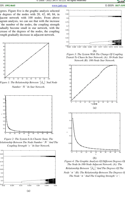
Figure 1 shows the relationship between ‘λ_N ’and

node number ‘ N ’in star network. Figure two

shows the relationship between node number‘N ’in

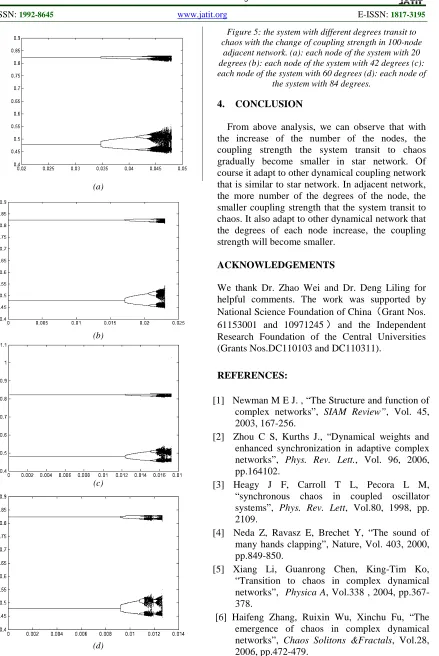
732 degrees. Figure five is the graphic analysis selected the degrees of the nodes with 20, 42, 60, 84, in adjacent network with 100 nodes. From above diagram analysis, we can see that with the increase of the number of the nodes, the coupling strength gradually become small in star network, with the increase of the degrees of the nodes, the coupling strength gradually decrease in adjacent network.

0 10 20 30 40 50 60 70 80 90 100 0

10 20 30 40 50 60 70 80 90 100

点点点 节

Figure 1: The Relationship Between ‘λ_N ’And Node Number ‘N’ In Star Network.

0 10 20 30 40 50 60 70 80 90 100 0

0.1 0.2 0.3 0.4 0.5 0.6 0.7 0.8 0.9 1

N

c

Figure 2: The System Is In Chaotic State, The Relationship Between The Node Number ‘N’ And The

Coupling Strength ‘c’ In Star Network.

(a)

(b)

Figure 3: The System With The Change Of Coupling Transit To Chaos In Star Network. (A): 30-Node Star

Network (B): 100-Node Star Network.

0 5 10 15 20 25 30 35 40 45 50

0 10 20 30 40 50 60 70 80 90 100

点 点点

节

(a)

0 5 10 15 20 25 30 35 40 45 50 0

0.05 0.1 0.15 0.2 0.25

n

c

(b)

Figure 4: The Graphic Analysis Of Different Degrees Of The Node In 100-Node Adjacent Network. (A): The Relationship Between ‘ λ_N ’And The Degrees Of The Node ‘n’ (B): The Relationship Between The Degrees Of

733 (a)

(b)

(c)

(d)

Figure 5: the system with different degrees transit to chaos with the change of coupling strength in 100-node

adjacent network. (a): each node of the system with 20 degrees (b): each node of the system with 42 degrees (c): each node of the system with 60 degrees (d): each node of

the system with 84 degrees.

4. CONCLUSION

From above analysis, we can observe that with the increase of the number of the nodes, the coupling strength the system transit to chaos gradually become smaller in star network. Of course it adapt to other dynamical coupling network that is similar to star network. In adjacent network, the more number of the degrees of the node, the smaller coupling strength that the system transit to chaos. It also adapt to other dynamical network that the degrees of each node increase, the coupling strength will become smaller.

ACKNOWLEDGEMENTS

We thank Dr. Zhao Wei and Dr. Deng Liling for helpful comments. The work was supported by

National Science Foundation of China（Grant Nos.

61153001 and 10971245）and the Independent

Research Foundation of the Central Universities (Grants Nos.DC110103 and DC110311).

REFERENCES:

[1] Newman M E J. , “The Structure and function of complex networks”, SIAM Review”, Vol. 45, 2003, 167-256.

[2] Zhou C S, Kurths J., “Dynamical weights and enhanced synchronization in adaptive complex networks”, Phys. Rev. Lett., Vol. 96, 2006, pp.164102.

[3] Heagy J F, Carroll T L, Pecora L M, “synchronous chaos in coupled oscillator systems”, Phys. Rev. Lett, Vol.80, 1998, pp. 2109.

[4] Neda Z, Ravasz E, Brechet Y, “The sound of many hands clapping”, Nature, Vol. 403, 2000, pp.849-850.

[5] Xiang Li, Guanrong Chen, King-Tim Ko, “Transition to chaos in complex dynamical networks”, Physica A, Vol.338 , 2004, pp.367-378.

734 [7] Wujie Yuan, Xiaoshu Luo, Pinqun Jiang,

Binghong Wang, Jinqing Fang, “Transition to chaos in small-world dynamical network”,

Chaos Solitons &Fractals, Vol.37, 2008,

pp.799-806.

[8] Guanrong Chen, Xiaofan Wang, Li xing, “Introduction to complex networks: Models, Structures and Dynamics”, Higher Education