Hmm dnn speech recognition techniques: a review

ORIGINAL RESEARCH ARTICLE

HMM-DNN SPEECH RECOGNITION TECHNIQUES: A REVIEW

*Pallavi Saikia

Assistant Professor, Gauhati University-Institute of Distance and Open Learning, Assam, India

ARTICLE INFO ABSTRACT

This paper presents a view about the HMM-DNN hybrid approach for speech recognition. Speech recognition is becoming an active research area in the field of computer science. Many researchers have developed a good deal of methods and techniques for speech recognition. A new trend is to use hybrid approaches for this particular task. One of this hybrid approaches is to use a combination of HMM-DNN and the result is found to be quiet successful. From study it has been found that the above approach outperforms the other traditional methods like GMM-HMM. This paper gives a basic idea about HMM and DNN model and then finally the use of HMM-DNN hybrid approach in different speech recognition techniques.

*Corresponding author:

Copyright ©2017,Pallavi Saikia.This is an open access article distributed under the Creative Commons Attribution License, which permits unrestricted use, distribution, and reproduction in any medium, provided the original work is properly cited.

INTRODUCTION

Speech recognition is the technique of recognizing spoken words, phrases or sentences by a machine using some algorithm. Research and experiments in speech recognition has helped us to interact with devices like car, watch, phone and tablets by simply giving directions through voice seamlessly. A speech recognition system involves the following tasks- speech capturing, pre-processing, feature extraction and recognition. Speech capturing is the process of acquiring speech for input through various devices like microphone etc. Speech signal is an analog signal which is converted to digital signal with the help of the sound card installed in the computer. After capturing the speech, we get a continuous set of samples which is farther pre-processed. Pre-processing a speech signal involves noise elimination from the signal and then passing it through different filters to get a clean signal. The clean speech signal is then divided into a block of equal sized frames. This is done to analyse the signal part by part as we know that speech signal is non-stationary and transitions take place frequently. The last step in pre-processing is windowing. In windowing process the signal is applied to a window function which is zero valued outside some defined

interval. This is actually done to eliminate the discontinuities found on the edges of the blocks because of the non-stationary characteristic of the speech signal. Feature extraction is a very important step as it extracts the features of the speech resulting in a set of feature vectors. This is done with the help of many different methods like Mel-Frequency Cepstral Coefficient (MFCC), Linear Predictive Coding (LPC) etc. The last step is recognition which consists of two phases- training and testing. The training phase comprise of teaching the system to distinguish between the different utterances of speech so that we may get a set of representatives to classify them into different classes. In training phase the utterances of the word are known as these is used to train the system. The testing phase consists of feeding the system with unknown utterances and to check whether it is able to match the pattern with any of the classes defined in the training phase. Speech recognition is implemented using different models like Gaussian Mixture Model (GMM), Hidden Markov Model (HMM), Deep Neural Network. In this paper we will study about the HMM and DNN model in the next two sections and finally we will talk about the hybrid approach i.e., HMM-DNN in the third section.

ISSN: 2230-9926

International Journal of Development Research

Vol. 07, Issue, 07, pp.14068-14072, July,2017

Article History:

Received 27th _{April, 2017}

Received in revised form

19th _{May, 2017}

Accepted 26th _{June, 2017}

Published online 31st _{July, 2017}

Citation: Pallavi Saikia.2017. “Hmm-dnn speech recognition techniques: a review”, International Journal of Development Research, 7, (07), 14068-14072.

ORIGINAL RESEARCH ARTICLE Open Access

Keywords:

Hidden Markov Model

Hidden Markov model is widely used in speech recognition due to its ability to represent the time-varying aspect of speech signal. The origin of HMM is the famous Markov chain of probability theory which can be used for sequential modelling. HMM is a finite state automaton which has a finite number of states through which the machine makes transition from one state to another state. It also has a finite set of input and output symbols. When a machine is at state s at time instant t, depending upon the input symbol provided, it will transit to another state emitting a certain output with a certain probability at the next time instant. Four factors are associated with a HMM:

H- set of hidden states V -set of visible states

aij – transition probabilities corresponding to the visible states bjk – emission probability of the visible state from the hidden states

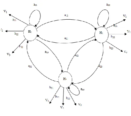
This can be understood easily with the help of the figure given below:

Figure 1. HMM Model

In the figure, H1, H2 and H3 are three hidden states and V1,V2,V3 are visible states. In any hidden state the machine may emit any one of the visible states. Here a12 is the state transition probability from hidden state H1 to H2. The machine may transit from one state to another state or may remain in the same state. For example a11 is the transition probability of H1 remaining in the same state. In general the state transition is shown as:

Hi(t-1) Hj(t)

Again b11 is the emission probability of the hidden state H1 if it emits visible state V1. We can say that bjk is the state emission probability of the visible state Vk if the machine is in state Hj and can be written as

P(Vk | Hj) = bjk

Finally from the above explanation we can conclude that

i.e. at any state the machine emits a state transition probability to any other state and also

i.e. at any state the machine emits a state emission probability to any other visible state.

As in an automaton, in HMM once the machine reaches an accepting state it cannot go back to an earlier state or come out from that state and can emit only one visible state.

Thus there are three central issues that need to be addressed in HMM:

Evaluation: If we are given an HMM model Θ with the hidden states H, visible states VT, state transition probabilities aij and the state emission probabilities bjk the problem is to find

P(VT | Θ )

i.e. what is the probability that VT is generated by the HMM model Θ. The Evaluation problem is implemented using Forward Algorithm.

Decoding: Decoding problem is to find out which sequence of hidden states HT has most likely generated the sequence of visible states VT

HT → VT

The Decoding problem is implemented using the Viterbi algorithm.

Learning: Learning problem is to find out aij , bjk i.e. the state transition and emission probabilities respectively, given the HMM model Θ with the hidden states H and visible states VT along with a set of training sequences. The Learning problem is implemented using Baum-Welch algorithm.

Deep Neural Network

architecture. The term “Deep” refers to the number of the hidden layers. Usually when we say Deep neural network, we mean that there are a number of hidden layers other than one or two. Let us now understand how deep neural networks work. Deep neural networks can be defined as a multilayer perceptron (MLP) with a number of hidden layers between the inputs and outputs. The hidden layers are the main computing elements which are usually connected in a feed forward way.

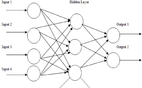
Each neuron in one layer has direct connections to all the neurons of the subsequent layers. The states of all the neurons are determined by the states of the neurons below them and the interconnected weights. In figure 2a the input layers, hidden layers along with the output layers are shown. There are four input units, three hidden units and produces two output units. In figure 2b a1,a2,...an are the input units and w1,w2,...wn are the weights associated with it.

Figure 2(a) Structure of a Multilayer Perceptron

The total input received by the neuron is the sum of the products of inputs and their corresponding weights i.e

This input is then passed through a filter which is often called an activation function, squash function or transfer function and produces an output which is greater than a certain threshold. There are many types of activation function such as Signum function, Sigmoidal function and hyperbolic tangent function. Here sigmoidal function is being used.

Each hidden unit j uses a logistic function to map its total input from the layer below aj to the scalar state zj that it sends to the layer above.

where bj is the bias of unit j, i is an index over units in the layer below and wij is the weight on a connection to unit j from unit i in the layer below.

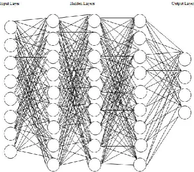
Figure 3. Deep Neural Network Architecture

In Deep Neural Network there are often many hidden layers in between input and the output layer. Each layer may have a large number of units and the units of every layer will have connections with every unit of the layer above it. The first phase of DNN consists of training the system with the data given, to learn the features or characteristics to classify them according to their traits. These training or learning can be done using supervised, unsupervised or reinforced learning methods. Supervised learning is the most widely used method. It can be considered as learning through examples or learning in presence of a teacher. Supervised learning is usually implemented using Backpropagation algorithm in DNN. Once the system has been trained, it can now be able to classify unknown data by the knowledge it has gained through the training phase. This is done by comparing the discrepancy between the current output and the target output which it has gained through learning. Based on the value of the difference or more precisely the error, the system adjusts or modifies its input to obtain the defined target output by using different activation functions.

HMM-DNN Model

The hybrid HMM-DNN approach in speech recognition make use of the properties like the strong learning power of DNN

and the sequential modelling activity of the HMM. As DNN accepts only fixed sized inputs it will be difficult to deal with speech signals as they are variable length time varying signal. So in this approach HMM deals with the dynamic characteristic of the speech signal and DNN is responsible for the observation probability. Given the acoustic observations, each output neuron of DNN is trained to estimate the posterior probability of continuous density HMM’s state. DNN when trained in the usual traditional way through supervised manner does not produce good results and very difficult to get to an optimal point. When a set of data is given as input, importance should be given to extract the variety of data than the quantity of data extracted because later on a good classification can be made from this data. For these reasons, another type of deep learning architecture, Deep Belief Network(DBN) is used to pre-train a DNN.DBN is one type of DNN consisting of multiple layers of hidden units having connections in between layers but not in between the units of the layers as in DNN. DBN when trained in an unsupervised manner can act as feature detectors for the inputs given which can be further used for classification if trained in a supervised manner. The unsupervised training is usually carried out using Restricted Boltzmann Machine followed by the Backpropagation method which is a supervised learning rule. In the next section we give a review of some papers where this hybrid approach is being used.

Literature Review

DBN was used to estimate the posterior probabilities of the senones given the set of acoustic vectors. Pre-training was carried out using Restricted Boltzman Machine which is an unsupervised training method. Here a comparison study was made between the traditional GMM-HMM and the new DBN-HMM on context dependent speech. The parameters used for comparison were maximum likelihood (ML), maximum mutual information (MMI) and minimum phone error (MPE). The features used in this experiment include the 13 dim static Mel-frequency cepstral coefficients and its first and second derivatives. This work was carried out to first recognize senones at each frame and later on it was extended for continuous speech recognition. Comparatively using the above parameters DBN-HMM proved much better result than GMM-HMM. From this paper it can be concluded that adding layers in DBN improves performance but too many layers might diminish the performance.

Roman Serizel, Diego Giuliani[III]. In this paper DNN-HMM is used for children and adult’s speech recognition. Here two different corpuses are taken for training DNN in two ways. The first way is to train DNN using group specific data. Here training is done separately each for children and adult taken from two different database ChildIt and APASCI respectively. The APASCI database can be further divided again into male and female speakers. The second way is to train DNN with all the data available together i.e. ChildIt + APASCI. DNN is used to find the acoustic variability caused due to the difference in age and gender and HMM is used to estimate the state emission probabilities. Here DNN uses MFCC computed on 20 ms window with 10 ms overlap for feature extraction. The pre training and post training is carried out using the unsupervised learning rule Restricted Boltzman Machine and Supervised learning rule Back Propagation algorithm respectively. This paper concludes that DNN trained on group specific data exhibit a poor performance compared to group independent data. The parameter PER is used for comparison of results for both the data and it was found that DNN training with all the data available produces far good result then the earlier technique which trained the DNN using group specific data. Hui Zheng, Feilong Bao, Guanglai Gao[V]. In this paper Mongolian speech is being recognized using DNN-HMM. The task is divided into three stages. Each stage recognizes different units of speech. First phoneme level is considered which helps in recognizing words and finally the recognized text is the output. The acoustic features are being represented using Fourier Transform based log filter bank coefficients. After obtaining the acoustic features, DNN ascribe scores for each acoustic feature which designates the probability of the acoustic feature is generated by a HMM state. Finally HMM decoding phase uses these scores. DNN takes as input a window of frames of real-valued acoustic coefficients. The output layer consists of a softmax layer that contains one unit for each possible state of each HMM. The DNN is designed to forecast the HMM state that relates to the central frame of the respective input window. Here a baseline GMM-HMM system is used to obtain these targets to produce a forced alignment. The implementation of this system is done using Kaldi speech recognition toolkit. This system is compared with the traditional GMM-HMM model and obtains word correct recognition rate of 87.63% in the test set. It can be concluded that filter bank coefficients are better than MFCC coefficients and also the input context of DNN is much larger than that of GMM thus making DNN a more accurate and powerful classifier.

Conclusions

In this paper we studied about the DNN-HMM model and its application in different speech recognition techniques.DNN is considered as an accurate classifier still, it cannot represent the acoustic feature without HMM’s contribution. DNN is popular because it can capture the non-linearity features but it is comparatively slow and takes a lot of time to converge to an optimal point. The factors like which feature extraction model to be used, learning rule to be applied, the size of the input data, the number of layers in DNN, and also the number of units per layer are very important in carrying out the experiments. Pre-training DNN with DBN improves performance of the system and hence gives optimal results. DNN can also be pre-trained using auto encoders. Though Backpropagation provides fair results but exhibits poor performance if randomly initialized. In such cases pre-training is used which makes later the fine-tuning job easy and better. However DBN which is an unsupervised learning rule is not necessary if we have an ample amount of labelled data for training. Automatic Speech Recognition systems using DNN-HMM for some language has been developed but still there are a lot of languages to be experimented. While recognizing speech of a particular language the type of the vocabulary set taken is a challenging issue. For a wide variety of application the vocabulary set taken should be large enough. DNN performs better in general data then group specific data while recognizing speech from different speakers of different ages and gender. Further research can be done using DNN-HMM using different feature extraction models to enhance its performance and also applying the different deep architectures like convolution neural network, recurrent neural network. Though DNN-HMM along with some other techniques has been used in a wide range of applications here we have remain confined to only speech recognition using pure DNN-HMM.

REFERENCES

Biswas, P.K. 2014. Pattern Recognition and Applications. Retrieved from http://nptel.ac.in/courses/117105101/38. Dahl, G.,Y, D., Deng, L. & Acero, A. Large vocabulary

continuous speech recognition with context-dependent DBN-HMMS. 2011-05, 2011 IEEE International Conference on Acoustics, Speech and Signal Processing (ICASSP).

Rajasekaran, S., Pai, Vijayalakshmi, G.A. 2015. Neural Networks, Fuzzy Logic and Genetic Algorithms. Delhi: PHI learning Private Limited.

Serizel, R., Giuliani, D. 2014. Deep neural network adaptation

for children's and adults' speech recognition, Proceedings

of the First Italian Conference on Computational Linguistics,2014, (Italian Conference on Computational Linguistics,Pisa, Italy,9-10 December 2014).

Yu, D., Deng, L., Dahl, G. 2010. Roles of pre-training and fine-tuning in context-dependent DBN-HMMs for real-world speech recognition. In: Proceedings of the Neural Information Processing Systems Workshop on Deep Learning and Unsupervised Feature Learning.

Zhang, H., Bao, F., Gao, G. 2015. Mongolian Speech Recognition Based on Deep Neural Networks. In: Sun M., Liu Z., Zhang M., Liu Y. (eds) Chinese Computational Linguistics and Natural Language Processing Based on Naturally Annotated Big Data. Lecture Notes in Computer Science, vol 9427. Springer, Cham