Optimal preview control for a class of linear continuous time large scale systems

Citation:

Liao, F and Wang, Y and Lu, Y and Deng, J (2017) Optimal preview control for a class of linear continuous-time large-scale systems. Transactions of the Institute of Measurement and Control, 40 (14). pp. 4004-4013. ISSN 0142-3312 DOI: https://doi.org/10.1177/0142331217740946

Link to Leeds Beckett Repository record: http://eprints.leedsbeckett.ac.uk/5627/

Document Version: Article

The aim of the Leeds Beckett Repository is to provide open access to our research, as required by funder policies and permitted by publishers and copyright law.

The Leeds Beckett repository holds a wide range of publications, each of which has been checked for copyright and the relevant embargo period has been applied by the Research Services team.

We operate on a standard take-down policy. If you are the author or publisher of an output and you would like it removed from the repository, please contact us and we will investigate on a case-by-case basis.

Optimal Preview Control for a Class of Linear Continuous-Time Large-scale Systems

Fucheng Liaoa* , Yu Wanga, Yanrong Lua and Jiamei Dengb

a_{School of Mathematics and Physics, University of Science and Technology Beijing,} Beijing 100083, China

b_{Leeds Sustainability Institute, Leeds Beckett University, Leeds, UK LS2 9EN} * Corresponding author. Email: [email protected]

Abstract

Keywords

Continuous-time large-scale systems, isolated subsystems, asymptotic stability, optimal preview control

1 Introduction

Preview control is a control method to improve the tracking accuracy of a system via utilizing the known future information of desired reference signal. The scientific community began a journey for exploring the preview control since Sheridan (1966), who put forward the concept for the first time, and then theoretical results with respect to preview control theory have been formed after more than 50 years of research and

development. There are some early efforts such as Bender (1968), Tomizuka (1975), Katayama et al. (1985), Katayama et al. (1987) and Takeshi et al. (1994). Certainly, the preview control for linear systems with constant coefficients was studied thoroughly

(Katayama et al., 1985, Katayama et al., 1987, Zhang et al., 1996 and Li et al., 2002),

and the robust preview control was also concerned (Tomizuka, 1996 and Lee et al.,

1996). In the last decade, when combining with other control theories, preview control was discussed deeply for multi-rate systems (Liao et al., 2003), time-varying systems

(Liao et al., 2015), and also descriptor systems (Zhao et al., 2016). Alternatively, some

problems on H_ optimal preview control were addressed (Kojima, 2015 and Kojima et al., 2003).

systems which are characterized by large scale, complex structure, numerous influencing factors and comprehensive functions. Many practical systems, e.g., multiarea power system, coupled water reservoirs, nuclear power systems and processes

in the chemical and petroleum industry (see, Lunze, 1992, Michel et al., 1977), can be

considered as large-scale systems. A key method for analysis and design of large-scale systems is decomposition-aggregation, which can not only decrease parametric complexity and the computational difficulties that significantly grow as the scale of the

systems increase, but also make us have a clear view over the effect of different factors

on the behavior of the whole system (see, Araki, 1978).In fact, large-scale systems can

be considered as the systems that consist of several isolated subsystems with connection

to other subsystems. By devising controller for each isolated subsystem, the controller for the large-scale systems is obtained by integrating subsystem controllers. And if the correlation matrices satisfy certain constraints, the closed-loop large-scale systems would have the required properties (Shi et al., 1992 and Michel et al., 1977). To be more exact, if each of the isolated subsystems is stable, and the norms of the correlation

matrices are small enough, then the large-scale systems are stable as well.

Because of the interconnective matrices between subsystems, stability analysis has

become one of the most important requirements for large-scale systems. During the past

several years, many methods have been established for this issue, such as M-matrix

method (Araki, 1978), piecewise Lyapunov method (Zhang et al., 2008), etc. Recently,

small gain theorem was used to study robustness problem of large-scale systems. In

(Duan et al., 2004), linear matrix inequality conditions were provided for this problem.

In (Dashkovskiy et al., 2012, Liu et al., 2011), input-to-state stability Lyapunov

controller design, decentralized control is a main research field of large-scale systems,

which is also acknowledge as the effective method to overcome the increasing size and

computational complexity of the mathematical models describing large-scale systems.

Shi et al. (1992) designed decentralized controller for model-following problem under

the scenario that the bounds of the interconnections were known or unknown,

respectively. When considering the interconnections between the subsystems as

uncertainties, Labibi et al. (2002) designed a decentralized controller for large-scale

systems via minimizing weighted sensitivity functions. Based on parameter-dependent

Lyapunov function, Duan et al. (2008) utilized linear matrix inequality to devise the

decentralized controller that can reduce the design conservation. In (Zhang et al., 2008),

the authors considered the problem of H_ decentralized controller design for

discrete-time fuzzy large-scale systems, and analyzed the stability by using piecewise

Lyapunov functions.

As pointed out in (Moelja et al., 2006), all or parts of the reference signals are

known in advance in certain systems. However, to the best of our knowledge, many

controller design methods for trajectory tracking of large-scale systems do not take the

preview information into account (see, e.g., Lunze, 1992, Ruan et al., 2005, Ruan et al.,

2008). Due to the fact that preview information of reference signal can be applied to

improve tracking accuracy effectively, this paper is concerned with the optimal preview

tracking control for a class of linear continuous-time large-scale systems. This paper has

the following two novel features. The first is to express the reference signal as a new

form similar to convex combination, where the number of items in combination is equal

then it can be observed from formula (2) that the tracking problem of the whole

large-scale system can be converted into several tracking problems of low dimensional

subsystems. The second is to exploit decomposition method to obtain isolated

subsystems, and meanwhile apply state augmented technique to further translate the

tracking problems into optimal regulation problems of several isolated augmented

subsystems. When the norms of the associated matrices satisfy certain bounds, the

optimal preview controllers are robust to the associated matrices. As a result, the

optimal preview controller is designed easily for each of the isolated augmented

subsystems by using standard optimal preview control theory, these controllers also

constitute the controller of the whole large-scale system. In addition, in order to ensure

stability of the whole closed-loop large-scale system, Lyapunov stability theorem and

M-matrix is employed to determine the norm bounds of associated matrices. Finally, a

numerical example is given to illustrate the effectiveness of the proposed design

method.

Notations. ( )A and _max( )A donate the eigenvalue and the maximum eigenvalue of matrix A, respectively. Q0 (Q0) donates that symmetric matrix

Q is positive definite (positive semi-definite). I_n denotes an n n identity matrix. 2 System Description





1 1 12 1 1 1 1

2 21 2 2 2 2 2

1 2 1 2 1 2 ( ) ( ) ( ) ( ) ( ) ( ) ( ) ( ) ( ) ( ) ( ) ( ) ( ) s s

s s s s s s s

s s

x t A A A x t B u t

x t A A A x t B u t

x t A A A x t B u t

x t x t

y t C C C

x t                       _    _                                                      or 1 ( ) ( ) ( ) ( ) ( ) ( ) s

i i i ij j i i

j j i i i i

x t A x t A x t B u t

y t C x t    _{  }     



, i1, 2, ,s (1a)

where ( ) ni, ( ) mi

i i

x t R u t R and y ti( )Rp are state vector, input vector and

output vector of the ith subsystem, respectively. Besides, 1 s i i n n  



, 1 s i i m m  



. , i i

A B and C_i are constant matrices with appropriate dimension. A_ij is an associated matrix between the jth subsystem and the ith subsystem

(i j i j; , 1, 2, , )s .The output of large-scale systems (1) is

1 ( ) ( )

s i i

y t y t







(1b)

A1. Suppose ( ,A B_{i i}) is stabilizable and matrix

0 i i i A B C

 

 

  is of full row rank

(i1, 2, ,s);

A2. Suppose (C A_i, _i) is observable (i1, 2, ,s);

A3. Suppose r t( ) is a piecewise-continuously differentiable function satisfying lim ( )

tr t r, lim ( )tr t 0, where p

rR is a constant vector. Moreover, r t( ) is previewable and the preview length is l_r. In the sense that the future values r( ) (t   t lr) are available at each instant of time t and suppose ( )r r t( l_r) at the time   t l_r.

The tracking error is defined as follows: ( ) ( ) ( ) e t  y t r t .

Our objective is to design a controller with preview compensation such that the

output of systems (1) can track the reference signal asymptotically, i.e.,





lim ( ) lim ( ) ( ) 0 te t t y t r t  .

Owing to the fact that large-scale systems have such character with large scale,

1 ( ) ( )

s i i

e t e t







,

where

( ) ( ) ( )

i i i

e t y t r t (2)

with _i satisfying _i 0 and 1

1 s

i i









. Here, we consider each _ir t( ) as a

virtual reference signal.

In fact, for arbitrary i{1, 2, , }s , if lim ( )_i 0 te t  , then





1 1

lim ( ) lim ( ) lim ( ) 0

s s

i i

t t t

i i

e t e t e t

  _{ } 

 

 _{ } 









.

On the basis of above considerations, we decompose large-scale systems into several isolated subsystems based on decomposition-aggregation method, and design controller for each isolated subsystem to build up the controller of the large-scale systems. Regarding the influence of correlation on stability of the close-loop system, this paper will give sufficient conditions to ensure that the output of large-scale

systems (1) asymptotically tracks the reference signal r t( ) byrequiring that the total

Briefly speaking, when the output y t_i( ) of each subsystem can track _ir t( ) without static error, the output y t( ) of system (1) can track the reference signal

( )

r t accurately.

3 Construction of the Augmented Large-scale Systems

In what follows, for a given virtual reference signal _ir t( ), we will consider the optimal preview tracking problem of the following isolated subsystem

( ) ( ) ( )

( ) ( )

i i i i i

i i i

x t A x t B u t y t C x t

 



 _

 (3)

where tracking error is (2).

To obtain the optimal preview controller of system (3), we introduce following quadratic performance index

0 ( ) i ( ) ( ) ( )

i i e i i i i

J 



_e t Q e t u t R u t _dt, (4) where 0

i e

Q  , R_i 0.

Noting that corresponding performance index of system (3) contains the derivative of the input u t_i( ) rather than the input u t_i( ), we can introduce integral action into the final controller, which is good for eliminating steady-state error (Liao et al., 2003).

desirable to construct an augmented system for each isolated subsystem. To avoid repeating, we construct the augmented system for systems (1) and let all associated matrices be zeros to gain the desired result.

For a given i i( 1, 2, , )s , derivating both sides of (1) and (2) gives

( ) ( ) ( ) ( ) ( )

i i i i i i

e t  y t r t C x t r t . (5)

1

( ) ( ) ( ) ( )

s

i i i i i ij j

j j i d

x t A x t B u t A x t

dt 



  



. (6)

Letting (t) (t) (t)

i

i p n

i i e z R x    _{ }

  yields

1

( ) ( ) ( ) ( ) ( )

( ) ( ) ( )

s

i i i i i ij j i

j j i

i i i

z t A z t B u t A z t D r t

e t C t z t

   _{   }     



(7) where 0 0 0 0

, , , C 0 ,

0

0 0

i i p

i i i i p ij

ij

i i

C I

A B D I A

A A B          _{ } _{ } _{ } _{ } _{    }        .

They are (p n _i) ( p n _i) , (pn_i)m_i , (pn_i)p , p(pn_i) and (p n i) ( p n i) matrices, respectively.

Write (7) as a compact form, i.e.,

( ) ( ) ( ) ( )

z t  Az t Bu t Dr t (8)

1 2 ( ) ( ) ( ) ( ) s z t z t z t z t              ,

1 12 1

21 2 2

1 2

s s

s s s

A A A

A A A

A

A A A

      _{ }       , 1 2 ( ) ( ) ( ) ( ) s u t u t u t u t              , 1 2 0 0 0 0 =

0 0 _s

B B B B               , 1 2 0 0 0 0 =

0 0 s

D D D D               .

Then system (8) is the desired augmented system.

Letting A_ij=0(i j i j; , 1, 2, ,s), then the ith isolated augmented subsystem is

( ) ( ) ( ) ( )

i i i i i i

z t  A z t B u t D r t (9)

With the related variables of (9), the performance index in (4) is modified into the following form

0 ( ) i ( ) 0 ( ) ( ) ( ) ( )

i i i x i i i i i i i

J  J



_x t Q x t _dt



_z t Q z t u t R u t _dt (10)

where 0 0 i i e i x Q Q Q       

 , Qxi 0.

4 Main Results

conditions to guarantee the asymptotic stability of the closed-loop system of system (8). 4.1 Design of Optimal Preview Controllers for the Isolated Augmented Subsystems

The following lemma is obtained immediately by Liao et al. (2011).

Lemma 1: If ( ,A B_{i i}) is stabilizable and (Q_i1 2,A_i) is detectable, then the optimal control input of system (9) under performance index (10) is given by

1 1

( ) ( ) ( )

i i i i i i i i

u t  R B P z t  R B g t  (11)

where (ni p) (ni p) i

PR    is a symmetric positive semi-definite solution to the algebraic Riccati equation

1

0 i i i i i i i i i i

A P P A PB R B P  Q  (12)

( ) p i

g t R is the function satisfying

0

( ) lrexp( ) ( )

i ci i i

g t  



A PD r t  d (13) where

1 ci i i i i i

A A B R B P  . (14)

4.2 The Closed-loop Stability of the Augmented Large-scale Systems

Based on the idea of decomposition-aggregation and the control inputs expressed by formula (11)，we introduce a vector

1 2 ( ) ( ) ( ) ( ) s u t u t u t u t              (15)

which happens to be the control input of system (8).

Substitute formulas (11) and (15) into system (8), then a closed-loop system is obtained

( ) ( ) ( )

z t  z t  t , (16)

where  and ( )t are

1 12 1

21 2 2

1 2

c s

c s

s s cs

A A A

A A A

A A A

       _{ }       , 1 2 ( ) ( ) ( ) ( ) s t t t t                  .

Matrix Aci, the diagonal elements of matrix , is given by formula (14). i( )t is 1

( ) ( ) ( )

i t B R B g ti i i i D r ti

 _{ }   _

and g t_i( ) is given by formula (13).

Upon the foundation of Lemma 1, the sufficient conditions for asymptotic stability of system (16) are obtained.

(1) ( ,A B_{i i}) is stabilizable and (Q1 2_i ,A_i) is observable;

(2) inequality

2 ij i ij

l

P A  (i j i j; , 1, 2, ,s) holds;

(3) matrix

1 12 1

21 2 2

1 2

s s

s s s

l l

l l

D

l l

 





 

 _ 

 



 

 _ 

 

(17)

is stable, then the zero solution of system (16) is asymptotically stable, where _i is given by  _i= _max_ Q_i PB R B P_{i i i}1 _i _i_(i1, 2, ,s).

Proof. the proof can be found in Appendix.

Now the asymptotic stability of system (16) implies lim ( )_i 0

te t  , thus

lim ( ) 0 te t  .

Namely, under the conditions given by Theorem 2, system (1) can track the reference signal r t( ) without static error.

Remark 2: If i x

Q is further required to be positive definite in the performance index function (10), then Q_i is also positive definite, and as a direct result,

1 2

straightforward consequence of Theorem 1 is that Corollary 1: Suppose

(1) ( ,A B_{i i}) is stabilizable and Q_i 0;

(2) inequality

2 ij i ij

l

P A  (i1, 2, ,s) holds;

(3) matrix D is stable in (17),

then the zero solution of system (16) is asymptotically stable where  _i= _min(Q_i) (i1, 2, ,s).

4.3 Discussion of Stabilizability and Observability

In what follows, we need to discuss the conditions that can guarantee the stabilizability (controllability) of ( ,A Bi i)and the detectability (observability) of

1 2 (Qi ,Ai).

Theorem 2: The sufficient and necessary conditions for the stabilizability (controllability) of ( ,A B_{i i}) arethat ( ,A B_{i i}) is stabilizable (controllable) and matrix

0 i i i

A B

C

 

 

  is of full row rank (i1, 2, ,s).

Proof. Noting the structure of matrices A_i and B_i, the theorem is a direct conclusion of [5].

Theorem 3: If 0 i e

observability of matrix (Qi1 2,Ai) is that matrix 1/ 2 i i i x A I C Q            

is of full column rank for

all complex .

Proof. The Popov-Belevitch-Hautus (PBH) rank test is used to prove the theorem [11].Noting that

1/ 2 1 2 1/ 2 0 0 0 i i i i i e i x I C A I A I Q Q Q        _     _{ }   _{  }  _{  }     .

Because of 0 i e

Q  , we take elementary transformation and get

1 2

1/ 2 1/ 2

0 0 0 0 0 0 0 0 i i i i i i i i x x C I

A I A I

A I I C Q Q Q         _   _     _{   }     _{   }   _{   }         .

It is well known that elementary transformation does not change the rank of a matrix.

Therefore, for any complex , i _{1 2} i A I Q      

  has full column rank if and only if

1/ 2 i i i x A I C Q            

has full column rank, which is exactly the conclusion of Theorem 3 based

on PBH rank test.

Corollary 2: Letting 0 i e

Q  . If (C A_i, _i) is observable, then 1 2

(Q_i ,A_i) is observable. In particular, if also 0

i x

Q  under the foundation of 0 i e

Q  , then the sufficient and necessary condition for the observability of matrix (Qi1 2,Ai) is that

(C Ai, i) is observable. Corollary 3: If 0

i e

Q  and 0

i x

Q  , then (Q1 2i ,Ai) is observable. 4.4 The Preview Controller of the Large-scale Systems

When the conditions of Theorem 1 hold, u t( ) is derived from formula (15) and the controller of systems (1) is gained as well. Therefore, we get the main theorem in this paper.

Theorem 4: Suppose

(1) A1-A3 hold;

(2) 0, 0

i

e i

Q  R  (i1, 2, ,s);

(3)

2 ij i ij

l

P A  (i j i j; , 1, 2, ,s);

(4) matrix D is stable in (17),

and let x t_i( )=0, u t_i( )=0, (i1, 2, ,s), r t( )0 for t0, then the optimal preview tracking of large-scale systems (1) is achieved by the following controller

1 2

( ) T( ) T( ) T_s( ) T

with

0

( ) ( ) ( ) ( )

i i

t

i e i x i i

u t  K



e  d K x t  f t

where 1

i i

e i i ie

K R B P  , 1

i i

x i i ix K R B P  and

i i

i ie ix

P  P P _, and the expression of ( ) p

i

f t R is given by 1 0

( ) lrexp( ) ( )

i i i ci i i

f t R B 



A PD r t  d . In matrix D , 1

max

i Qi PB R B Pi i i i i

 _{  }   _

  (i1, 2, ,s).

Proof. It follows from conditions (1) - (4) that Theorem 1 holds, namely, the zero solution of closed-loop system (16) is asymptotically stable. Therefore, as a

component of z t_i( ), e t_i( ) will tend to zero as time goes to infinity and so will e t( )

because of

1 ( ) ( )

s i i

e t e t







. That is to say, the output of large-scale systems (1)

achieves optimal tracking of reference signal r t( ) under controller (11). In order to

derive u t_i( ) from controller (11), we select an L satisfying Ll_r . Then, integrating (11) on interval [L t, ) yields controller (19).

Remark 3: As mentioned by Corollary 1, if Q_i 0, then _i of Theorem 4 can be change to _min(Q_i).

5 Numerical Simulation

2 1

( ) ( ) ( ) ( )

( ) ( )

i i i ij j i i

j j i i i i

x t A x t A x t B u t

y t C x t    _{  }     



1, 2 i

and its coefficient matrixcs are respectively









1 12 1 1

2 21 2 2

3 0 1 0 0.0001 1

0 1 1 , 0.0001 0.0001 , 1 , 1 1 0

2 0 2 0.0001 0.0002 1

1 0 0.0001 0.0002 0 1

, , , 0 1 .

1 2 0 0.0001 0.0001 1

A A B C

A A B C

             _  _ _  _  _{ }                      _{ } _{ } _{ }          ，

By verifying, ( ,A B_{i i}) is stabilizable, matrix

0 i i i A B C    

  is of full row rank and

(C A_i, _i) is observable(i1, 2). Thus, the system satisfies the basic assumptions in this paper.

Let the reference signal be

0 8

( ) 8, 8 9

1, 9

t

r t t t

t    _     _  ， .

Moreover, put the weight matrices in performance index function (10) be

1 1

50 0 0 0

0 0.005 0 0

=0.

0 0 0.005 0

0 0 0 0

Q R             

， 1, _{2 2}

50 0 0

0 0.005 0 =0.

0 0 0

Q R           

， 1.

positive definite solutions

1

23.9120 4.0678 5.1047 1.1991 4.0678 0.9338 1.2041 0.3605 5.1047 1.2041 1.5701 0.4751 1.1991 0.3605 0.4751 0.1883 P

 

 

 



 

 

 

, ₂

15.1280 0.1654 2.0707 0.1654 0.0257 0.0595 2.0707 0.0595 0.4318 P

 

 

  

 

 

,

and the gain matrices in controller (19) are





1 22.3607 , 1 6.3088 8.4108 3.0295

e x

K   K     ,





2 22.3607 , 2 0.8521 4.9134

e x

K  K  .

[image:22.595.163.424.158.368.2]

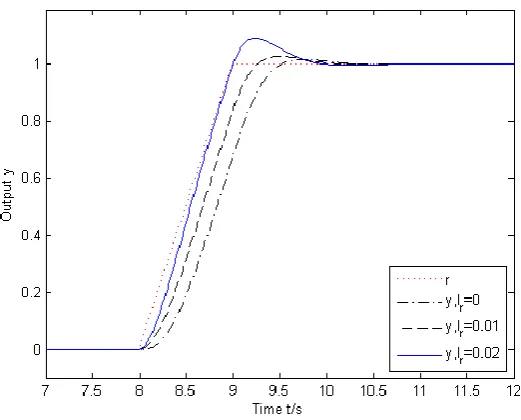
Figure 1. The output responses of the large-scale systems for different preview lengths

It is observed from Figure 1 that the output of large-scale systems (1) can track the

[image:23.595.143.457.138.633.2]

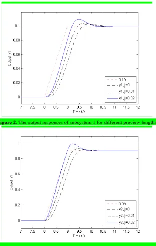
Figure 2. The output responses of subsystem 1 for different preview lengths

[image:24.595.125.468.137.636.2]

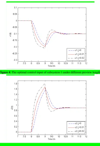
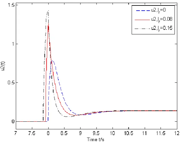
Figure 4. The optimal control input of subsystem 1 under different preview lengths

Figure 5. The optimal control input of subsystem 2 under different preview lengths

output of subsystem track the given virtual reference signal asymptotically. As a result, the tracking errors e t₁( ) and e t₂( ) will tend to zero as time goes to infinity. Combining with Figure 1 and formula (2), it indirectly proves the validity of the reduced-order design method proposed in this paper. Moreover, we can also find that the controller has the ability to accelerate the tracking speed. In addition, although the overshoot rises up gradually with moderate increase of the preview length, the tracking performance is improved and the settling time decreases as well.

Example 2. To further illustrate the efficiency of the designed controller. We

consider the optimal control problem that a large-scale system tracks a previewable

step reference signal. The dynamics of the subsystems are described as follows

2

1

( ) ( ) ( ) ( )

( ) ( )

i i i ij j i i

j j i

i i i

x t A x t A x t B u t y t C x t

   _{  }     



, i1, 2 (19)

and the corresponding coefficient matrices are





1 12 1 1

2 21 2

1 1 1 0 0 0.01 0.01 1

0 1 1 , 0.01 0.01 0 0 , 1 , 0 0 0

1 0 0.5 0.01 0.02 0 0 0

3 1 0 0 0.01 0.02 0 1

2 2 0 0 0 0.01 0.01 1.6

, ,

0 0 1 2 0.01 0 0 1

3 5 0 2 0 0.01 0.02 0

A A B C

A A B

              _   _ _  _ _{ }                     _   _  _             _{  }        ，





2

,C 1 1 1 1.5 .

      _{ }      

0, 8 ( ) 1, 8 t r t t     _ 

and satisfies the assumption of preview in A1. That is to say, the value of r( ) is

available to large-scale systems (19) in interval



t t l,  _r



at time t.

Because of C₁



0 0 0



, the output of large-scale systems (19) is y t( ) y t₂( ). Therefore, the optimal preview tracking problem of large-scale systems (19) can be

decomposed into an optimal regulation problem of subsystem 1 and an optimal preview

tracking problem of subsystem 2.

Select the weight matrices associated with the performance index function (10) as

1 1

0.4 0 0

0 0.4 0 =0.4

0 0 0.4

x Q R           

， , 2

2

2 2

60 0 0 0 0

0 15 0 0 0 0

=0.3

0 0 3 0 0

0

0 0 0 9 0

0 0 0 0 6

e x Q Q R Q                  _{  }     ，

By applying PBH rank test, it can be calculated that ( ,A B_{i i}) is stabilizable, 1, 2

i , (C A₂, ₂) is observable. Moreover, routine calculation gives that matrix

2 2 2 0 A B C    

  is of full row rank. Noting that Qx1and Qe2 are positive definite matrices.

Then, according to the conclusions of Lemma1, Theorem 2, and Corollaries 2-3, we

know that the following algebraic Riccati equations have positive definite solutions:

1

1

1

2 2 2 2 2 2 2 2 2 2 0

A P P A P B R B P  Q 

Solving the above equations by Matlab gives

1

0.21764 0.01695 0.08644 0.01695 0.17222 0.07279 0.08644 0.07279 0.37225

P     _  _      , 2

16.98680 1.25749 1.74038 0.20054 2.32069 1.25749 6.39163 4.04398 0.27471 0.79782 1.74038 4.04398 4.14416 0.90008 1.14899 0.20054 0.27471 0.90008 2.35239 0.46133 2.32069 0.79782 1.14899 0.46133 1.82212

P     _              _{ }   ,

the control gain matrices in (18) are





1 0.58649 0.47293 0.03411

x

K  ,









2 14.14214 , 2 0.65325 5.62197 3.95656 5.00629

e x

K  K   .

We take

2 2 i ij

ij P A

l  , then

12 2 1 12 2=0.0189

l  P A

21 2 2 21 2=0.2620

l  P A

In addition,

1

1

1 max( 1 1 1 1 1) 0.4000 T

x

Q PB R B P

  

     

1

2 max( 2 2 2 2 2 2) 3.5864 T

Q P B R B P

  

     

By calculation, the eigenvalues of 0.4000 0.0189 0.2620 3.5864

D  _



3.5880

 , which indicate that D is stable. That is to say, the conditions (3) and (4) of

Theorem 4 hold. Hence, the optimal preview tracking of large-scale systems (19) can be

achieved by controller (18).

Let initial value be x₁(0)



0 0 0 ,



T x₂(0)



0 0 0 0



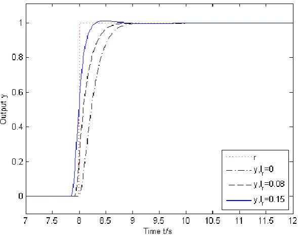
T. The simulation will be carried out for three situations, that is, the preview lengths of the reference signal are

0( ), 0.08( ) 0.15( )

r r r

[image:28.595.146.441.350.587.2]

l  s l  s，l  s , respectively.

[image:29.595.145.441.162.397.2]

Figure 7. The optimal control input of subsystem 2 under different preview lengths

Figure 6 shows the output responses of large-scale systems (19) under control input

(18). Figure 7 shows the optimal control input of subsystem 2. It is seen from Figure 6

that y t( ) can track the reference signal accurately whether preview information exists

or not. Furthermore, compared with the case that l_r 0( )s , it can be also observed from figures 6 and 7 that the controller with preview compensation can improve the

dynamic performance effectively, such as accelerating transient response, reducing

tracking error.

observability of the matrix (C A_i, _i) can ensure that (Q_i1 2,A_i) is observable. And _i should be  _i  _maxQ_iPB R B P_{i i i}1 _i _i_.

6 Conclusion

The optimal preview control problem for a class of linear continuous-time large-scale systems has been settled in this paper. Owing to the integral in the expression of control input (11), this paper has not constructed the Lyapunov function for the closed-loop large-scale systems directly, but for its corresponding homogeneous linear systems. Based on the stable conditions of the homogeneous linear systems and assumption A3, the sufficient conditions have been given to guarantee the global asymptotic stability of the closed-loop large-scale systems. The simulation example has illustrated the effectiveness of the designed controller. How to extend the current conclusions to the discrete-time large-scale systems setting is a future topic worthy of further investigation.

Conflict of Interests

The authors declare that there is no conflict of interest.

This work was supported by the National Natural Science Foundation of China [grant number 61174209].

Appendix (Proof of Theorem 1)

Proof. We first prove the asymptotic stability of the zero solution of system ( ) ( )

z t  z t (A1)

which is the homogenous linear system of system (16). When assumptions 1-3 hold, it follows from optimal control theory that the solution P_i of algebraic Riccati equation is positive definite if (Q1 2_i ,A_i) is observable. Using P_i to construct a function V z_i

 

_i z Pz_i _{i i}, then V_i is a positive definite quadratic form with respect to

i

z . Taking the total derivative of function V_i regarding t along the trajectory of system (18) gives

(18)

i i i i i i i V z Pz z Pz

1

( ) 2

s T

i i ci ci i i i i ij j j

j i

z P A A P z z P A z 



  



.

According to the expression of matrix A_ci, we get

1 1

( )

T

i ci ci i i i i i i i i i i i i i i i

P A A P  P A A P PB R B P  PB R B P  .

Because Pi is the solution of algebraic Riccati equation (12), the formula 1

i i i i i i i i i i

P A A P PB R B P   Q holds. Hence

1

max( ) max

T

i ci ci i i i i i i i i

P A A P Q PB R B P

 _{ } _{ }   _{ }

and thereby an estimation of (18) i V is 2 (18) 1 2 s

i i i i ij i j

j j i

V  z P A z z

 

  



1 s i i i ij j

j j i

z  z l z

       _  _    



, (i1, 2, , )s .

Furthermore,

1 (18)

1 1

2 ₍₁₈₎ 2 2

(18)

s s

s

V

z z

V z z

D z z V                    _{ }                         .

Now we turn to the key part of the proof. Noting that matrix D is a stable Metzler matrix, thus there exists a diagonal matrix K diag k k( ,_{1 2}, ,k_s), where

0 i

k  holds for any i1, 2, ,s, such that matrix KDD K is negative definite (Liao, 1985). Using the elements of matrix K, we construct a quadratic function





1 2 1 2 1 , , , s

i i s

i

s V V

V k V k k k

V               



,

and estimating its upper bound yields









1 (18)

1 1

2 ₍₁₈₎ 2 2

1 2 1 2

(18)

(18)

, , , s , , , s

s s

s

V

z z

V z z

V k k k k k k D

z z V                       _{   }                     1 2 1 , 2 , ,

2 s

s

z z

KD D K

z z z

z        _{ }  _{    }  _{  }     .

Because matrix KDD K is negative definite, then (18)

V is negative definite. According to Lyapunov stability theorem, the zero solution of system (18) is (globally) asymptotically stable.

Next, we need to prove lim ( ) 0

t t  . Noting that r t( ) will tend to zero as time goes to infinity (assumption A3), then based on the relationship between _i( )t and

( ) i

g t , it suffices to prove lim _i( ) 0

tg t  (i1, 2, ,s). Due to the stability of matrix ci

A, there exist constant scalars  0 and M 0 such that exp(A_ci) Me . Moreover, it follows from formula (14) that the inequality

0 0 0

( ) lr exp( ) ( ) lr ( ) lr ( )

i ci i i i i i i

g t 



A PD r t d



Me PD r t dM PD



r t d

holds, which, together with lim ( ) 0

Since the zero solution of system (18) is asymptotically stable and lim ( ) 0 t t  , the zero solution of system (16) is asymptotically stable (Chen, 2003). This completes the proof of Theorem 2.

References

Araki M (1978) Stability of large-scale nonlinear systems—quadratic-order theory of composite-system method using M-matrices. IEEE Transactions on Automatic Control 23: 129-142.

Bender EK (1968) Optimum linear preview control with application to vehicle suspension. ASME Journal of Basic Engineering 90: 213-221.

Chen WY (2003) On convergent properties for states of non-homogeneous linear systems. Journal of Tianjin University of Light Industry 18: 1-3.

Dashkovskiy SN, Rüffer BS and Wirth FR (2012) Small gain theorems for large scale systems and construction of ISS Lyapunov functions. In: proceedings of the 51st IEEE Conference on Decision and Control 4165-4170.

Duan ZS, Huang L, Wang L and Wang JZ (2004) Some applications of small gain

Duan ZS, Wang JZ, Chen GR and Huang L (2008) Stability analysis and decentralized control of a class of complex dynamical networks. Automatica 44: 1028-1035.

Katayama T and Hirono T (1987) Design of an optimal servomechanism with preview action and its dual problem. International Journal of Control 45: 407-420.

Katayama T, Ohki T, Inoue T and Kato T (1985) Design of an optimal controller for a discrete-time system subject to previewable demand. International Journal of Control 41: 677-699.

Kojima A (2015) H_ controller design for preview and delayed systems. IEEE Transactions on Automatic Control 60: 404-419.

Kojima A and Ishijima S (2003) H_ performance of preview control systems. Automatica 39: 693-701.

Labibi B, Lohmann B, Sedigh AK and Maralani PJ (2002) Output feedback

decentralized control of large-scale systems using weighted sensitivity functions

minimization. Systems & Control Letters 47(3): 191-198.

Lee HS and Tomizuka M (1996) Robust motion controller design for high-accuracy positioning system. IEEE Transactions on Industrial Electronics 43: 48-55.

Liao FC (1985) The stability of a type of linear system with variable coefficients. Journal of University of Science and Technology Beijing 4: 101-106.

Liao FC, Guo YJ and Tang YY (2015) Design of an optimal preview controller for linear time-varying discrete systems in a multirate setting. International Journal of Wavelets Multiresolution and Information Processing 13: 1550050-1—1550050-19. Liao FC, Takaba K, Katayama T and Katsuura J (2003) Design of an optimal preview

servomechanism for discrete-time systems in a multirate setting. Dynamics of Continuous Discrete and Impulsive Systems 5: 727-744.

Liao FC, Tang YY, Liu HP and Wang YJ (2011) Design of an optical preview controller for continuous-time systems. International Journal of Wavelets Multiresolution and Information Processing 9: 655-673.

Liu TF, Hill DJ and Jiang ZP (2011) Lyapunov formulation of ISS cyclic-small-gain in

continuous-time dynamical networks. Automatica 47: 2088-2093.

Lunze J (1992) Feedback control of large-scale systems. London: Prentice Hall.

Michel AN and Miller RK (1977) Qualitative analysis of large scale dynamical systems.

New York: Academic Press.

Moelja AA and Meinsma G (2006) H₂ control of preview systems. Automatica 42:

Sheridan TB (1966) Three models of preview control. IEEE Transactions on Human Factors in Electronics 7: 91-102.

Shi L and Singh SK (1992) Decentralized adaptive controller design for large-scale systems with higher order interconnections. IEEE Transactions on Automatic Control 37: 1106-1118.

Tsuchiya T and Egami T (1994) Digital preview and predictive control (translated by

Liao Fucheng). Beijing: Beijing Science and Technology Press.

Tomizuka M (1975) Optimal continuous finite preview problem. IEEE Transactions on Automatic Control 20: 362-365.

Tomizuka M (1996) Model based prediction, preview and robust controls in motion control systems. In: proceedings of the 4th international workshop on advanced motion control 1: 1-6.

Zhang H and Feng G (2008) Stability analysis and H_ controller design of

discrete-time fuzzy large-scale systems based on piecewise Lyapunov functions.

IEEE Transactions on Systems Man & Cybernetics--Part B 38(5): 1390-1401.

Zhang XM and Wang ZL (1996) Research of preview control method on robot. Journal of Beijing University of Aeronautics and Astronautics 22: 21-26.

Methods 37: 279-289.