Abstract—A Wiener model consists of a dynamic linear transfer function in series with a static nonlinear function. We can through the essences of GP, like robustness, domain independence and ability to search for satisfying solutions in solving complicated nonlinear problems, this study hoped that the evolved GP models could have a better applicability and accuracy of evaluations, and easily obtain the correct structure and parameters of the nonlinear function, and number of zeros and poles of the linear transfer function. GP is applied to the determine nonlinearity and unknown parameters in the nonlinear function and linear dynamic system model are estimated by a least square algorithm. The results of numerical studies indicate the usefulness of proposed approach to Wiener model identification.
Index Terms—Wiener model, system identification, Genetic Programming (GP), Akaike information criterion (AIC).
I. INTRODUCTION
The black box modeling based on the observed system input and output data for unknown dynamic system is called system identification. One of the difficulties in nonlinear system identification is that both the structure and the unknown parameters of model should be determined [1].
In [2], a fast method to get a first estimate of Wiener or Hammerstein systems has been introduced. However, methods must assume that the order of linear part is known and the search space is differentiable, and linear in the search parameters. In [3], Wiener model identification by evolutionary computation approach with piecewise linearization has been introduced. However, methods must assume that the nonlinear static part is invertible. Regarding these problems, we can use GP to improve.
Because GP exploit strategies of genetic information and survival of the fittest to guide their search, they need not calculate the gradient or assume that the search space is differentiable or continuous. GP simultaneously evaluate many points in the parameter space, so they are more likely to converge toward a global solution. The aim of system identification is to give the optimal mathematical model both
Y. C. L. is with the Department of Electronic Engineering, National Kaohsiung University of Applied Sciences, Kaohsiung, Taiwan 807, R.O.C. (e-mail: [email protected]).
M. H. C. is with the Department of Electronic Engineering, National Kaohsiung University of Applied Sciences, Kaohsiung, Taiwan 807, R.O.C. (e-mail: [email protected]).
T. J. S is with the Department of Electronic Engineering, National Kaohsiung University of Applied Sciences, Kaohsiung, Taiwan 807, R.O.C. (e-mail: [email protected]).
nonlinearity and linear dynamic system in an appropriate sense. We can use GP to determine the structure of nonlinear static block. The unknown parameters including linear dynamic system model's ones are estimated by the least square method.
Remainder of this paper is organized as follows. In section II, the expression tree is introduced. In section III, the Wiener model is introduced. Section IV describes our approach to the Wiener model identification and results of some numerical examples are shown in Section V. Finally, a conclusion is presented in Section VI.
II. EXPRESSIONTREE
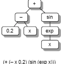
Each program or individual on the population is generally represented as a tree composed of functions and terminals appropriate to the problem domain. The function set may contain standard arithmetic operators, mathematical functions, logical operators, and domain-specific functions. The terminal set usually consists of variables and constants. The simple expression is represented as shown in Figure 1.
[image:1.595.361.490.488.623.2]where the function set is {+, -, sin, exp}, and the terminal set is {x, 0.2} [4].
Figure 1: An example of GP Tree
III. WIENERMODELIDENTIFICATION
A Wiener model consists of a linear dynamic system G followed by a static nonlinear part F as in Fig 2.
Wiener Model Identification using
Genetic Programming
Figure 2: A Wiener model.
Let consider the Wiener model
1 1 1 1
( )
( )
( )
( )
1
nb nb na nax t
G q u t
b q
b q
u t
a q
a q
(1)( )
( ( ))
( )
y t
F x t
e t
(2)Here q-1 is delay operator. y (t),u (t) and e (t) are the system output, input and measurement noise at time instant t respectively. The orders of linear dynamic block na and nb are unknown and it should be determined from observed input and output data.
F
( )
is unknown nonlinear function.We can rewrite (1) as,
1 1
( )
(
)
(
)
nb na
j i
j i
x t
b u t
j
a x t
i
(3)For the sake of convenience, again let:
1 1
( ,
,
, ,
,
)
Tna nb
a
a
b
b
( )
(
(
1),
,
(
), (
1),
, (
))
h t
x t
x t
na u t
u t
nb
According to Eq. (3), we have:( )
( )
x t
h t
(4)Suppose m represent sampling steps used to identify, let:
a b
n
n
n
,( )
t
( (1), (2),
x
x
, ( ))
x m
T
, (1)(2)
( )
(0) (1 ) (0) (1 )
(1) (2 ) (1) (2 )
( 1) ( ) ( 1) ( )
a b
a b
a b m n
h h H
h m
x x n u u n
x x n u u n
x m x m n u m u m n
Hence:
( )
t
H
(5)Parameters are identified by the least square criterion as [5]:
1
(
T)
T( )
H H
H
t
(6)
Then, we assume that nonlinear function is written by:
1
( )
( ( ))
( )
( ( ))
( )
Mk k k
y t
F x t
e t
p x t
e t
(7)Here, θk are model parameters and pk (.} are the suitably selected nonlinear functions.
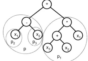
The function terms were determined by decomposing the tree starting from the root as far as reaching non-linear nodes (nodes which are not '+' or '-') [6] [7].
In Fig 3: The root nodeis a ’+’ operator, so it is possible to decompose the tree into two subtrees:’p’ and ’p1’ trees. The
root node of the ’p’ tree is again a linear operator, soit can be
decomposed into ’p2’ and ’p3’ trees. The root node of the ’p1’ tree isa nonlinear node (’*’) so it cannot be decomposed, so finally the decomposition procedure results in three
[image:2.595.337.511.225.346.2]subtrees: ’p1’, ’p2’ and ’p3’.
Figure 3: Decomposition of a tree to function terms
The parameters are assigned to the model after ’extracting’
the
p
i function terms from the tree. Least Squares Method can be used for the parameters identification.The optimal
[ , . . . ,
1
M]
Tparameter vector can be analytically calculated:-1
(
P P
T)
P y
T
(8)Where
y
[ (1), . . . , ( )]
y
y N
T is the measured output vector, and the P regression matrix is:1
1
( (1))
( (1))
( ( ))
( ( ))
M
M
p x
p
x
P
p x N
p
x N
(9)The compact matrix form corresponding to the linear-in-parameters model is
y
P
e
(10)where
P
is the regression matrix,
is the parameter vector, e is the error vector [8].Based on this representation, we can estimate unknown parameters, ai, bj andθk using the least square algorithm. The orders of this model, na, nb and M should be determined by AIC, which is defined by [9],
(
,
,
)
log( ) 2(
)
2
1
1
ˆ
( ( ) - ( ))
Nt
E
y t
y t
N
(12)Where, E is the mean square error between actual output and estimated output, N is the number of sample points.
This kind of models is investigated in many actual processes such as Control Valve, where the measurement device with nonlinear characteristics is a component of the system.
The Control Valve is an opening with adjustable area. Normally it consists of an actuator, a valve body and a valve plug. The actuator is a device that transforms the control signal to movement of the stem and valve plug.
where u(k) is the control pressure, x(k} is the stem position, and y(k) is the flow through the valve which is the controlled variable [10].
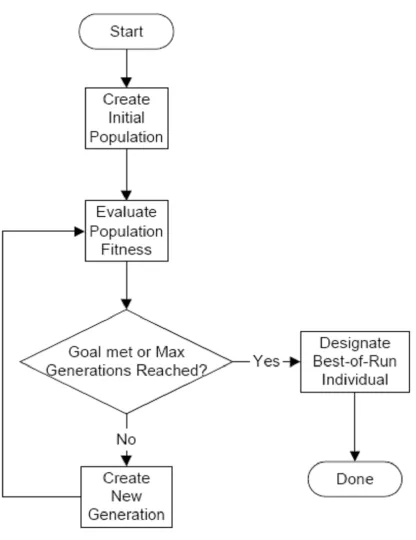
IV. THE FLOW CHART OFWIENER MODEL
[image:3.595.67.275.337.607.2]The flow chart of the Wiener model identification with GP is as follows:
Figure 4: flowchart of GP
A. Creation of initial population
Our chromosome consists of two parts, parameters of the nonlinear function and order of linear discrete transfer function. We generate one hundred initial chromosomes of random compositions of the functions and terminals according to this method.
B. Evaluate Population Fitness
The fitness function reflects the goodness of a potential solution which is proportional to the probability of the selection of the individual. The fitness for each individual is evaluated by AIC to balance the accuracy and the complexity
of model. AIC is calculated with the number of nodes in the GP tree, the order of linear dynamic model and the accuracy of model. The fitness for each individual is evaluated with the minimum AIC.
C. Keep the better chromosome
We arrange the chromosome according to the fitness function, and keep the first groups of better chromosome as the parental generation of the next generation.
D. Use Genetic Operation:
The genetic operations include crossover and mutation. After the genetic operations are performed on the current population, the new generation replaces the now-old generation. This iterative process of measuring fitness and performing the genetic operations is repeated over many generations. The run of GP terminates when the termination criterion is satisfied. Sometimes we can’t find the optimal solution quickly; therefore we can set up generation. We will stop the program when it reaches the generation, and select the best chromosome from inside.
V. EXPERIMENTRESULT
A. Experiment I
To show the validity of proposed approach to Wiener model, numerical simulation study is carried out.
Consider the following Wiener model [3]:
( ) 1.5 ( -1) - 0.7 ( - 2)
( -1) 0.5 ( - 2)
x t
x t
x t
u t
u t
(13)1
( )
1 exp{ ( )}
y t
x t
(14)Here, the nonlinear static part is invertible, measurement noise is a white noise normally distributed with mean zero, and the input signal u(t) is assumed random input uniformly distributed over [-1,1]. GP is used to determine a mathematical function form for the static nonlinear block. The design parameters in the GP are as follows.
Table I: Parameters of GP
terminal sets { x(t),
}function sets {+, -, *, exp, sinh, cosh, tanh}
Population size 100
generation 500
Max tree depth 6
Type of selection Tournament selection
Crossover rate 0.7
[image:3.595.304.548.596.777.2]Here
is constant. The identified linear dynamic system part is given by:ˆ
( ) 1.532 ( -1) - 0.692 ( - 2)
ˆ
ˆ
1.044 ( -1) 0.496 ( - 2)
x t
x t
x t
u t
u t
(15) [image:4.595.49.289.174.369.2]and the identified inverse function of nonlinear static part is shown in Fig. 5.
Figure 5: Estimated nonlinearity.
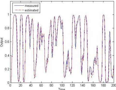
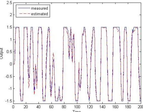
The output estimates
y(t)
ˆ
are shown with the observations y (t) in Fig 6.Figure 6: Output estimate and observation.
B. Experiment II
To show the validity of proposed approach to non-invertible static part, numerical simulation study is carried out.
Consider the following Wiener model:
( ) 1.5 ( -1) - 0.7 ( - 2)
( -1) 0.5 ( - 2)
x t
x t
x t
u t
u t
(16)1.5 ,
( )
1.5
( )
( ) , 1.5
( ) 1.5
1.5 ,
1.5
( )
x t
y t
x t
x t
x t
(17)
Here, the nonlinear static part is non-invertible, measurement noise is a white noise normally distributed with mean zero, and the input signal u(t) is assumed random input uniformly distributed over [-1,1]. The design parameters in the GP are represented as shown in Table I.
The identified system part is given by
ˆ
( ) 1.532 ( -1) - 0.692 ( - 2)
ˆ
ˆ
1.044 ( -1) 0.496 ( - 2)
x t
x t
x t
u t
u t
(18)ˆ
( ) 1.48 tanh( ( ))
ˆ
y t
x t
(19) [image:4.595.306.546.402.594.2]The estimated nonlinear function of nonlinear static part is given in Fig. 7.
Figure 7: Estimated nonlinearity.
[image:4.595.49.289.437.623.2]Figure 8: Output estimate and observation.
VI. SUMMARY
The GP is an effective algorithm to generate model structures from input-output data. Based on the GP method, methods needn’t to assume that the order of linear part is known and the search space is differentiable, and linear in the search parameters. In addition, methods also needn’t to assume that the nonlinear static part is invertible. Numerical simulation study result indicates the usefulness of the proposed approach to Wiener model identification. We can easily modify this approach for the other kind of nonlinear system models by selecting suitable nodes for GP.
References
[1] J. Sjöberg, Q. Zhang, L. Ljung, A. Benveniste et al, “Nonlinear black-box modeling in system identification: a unified overview,” Automatica. vo1.31, No. 1995, pp. 1691-1724.
[2] P. Crama and J. Schoukens, “First estimates of Weiner and Hammerstein systems using multisine excitation,”IEEE Instru and measurement technology conference, May 2001, pp.1365-1369.
[3] T. Hatanaka, K. Uosaki and M. Koga, “Wiener model identification by evolutionary computation approach with piecewise linearization,”
Systems, Man, and Cybernetics, IEEE International Conference
Volume. 3, 7-10 Digital Object Identifier 10.1109/ICSMC.2001.973479., vol.3, Oct. 2001, pp.1406– 1411. [4] S. Luke,“Issues in Scaling Genetic Programming: Breeding Strategies,
Tree Generation, and Code Bloat,” PhD thesis, Department of Computer Science, University of Maryland, A. V. Williams Building, University of Maryland, College Park, MD 20742 USA,2000. [5] F. Hao, Y. Shiming, W. Xingang and W. Shoujue, “System
identification method with denoising and disturbance-rejecting capability,” IEEE Region 10 Annual International Conference, Proceedings/TENCON, 2002, pp.1269-1272.
[6] C. Ferreira,“Gene expression programming: a new adaptive algorithm for solving problems,”Complex Syst, 2001, 13, pp. 87–129. [7] S. Sette and L. Boullart, “Genetic Programming: principles and
applicaionts,” Engineering Applications of Artificial Intelligence,
2001, 14, pp. 727–736.
[8] X. Hong and C. J. Harris, “Nonlinear Model Structure Design and Construction using Orthogonal Least Squares and D-optimality Design,” IEEE Transaction on Neural Networks, vol. 13, 2002, pp.
1245-1250.
[9] T. Soderstorm and P. Stoica, “System Identification. Prentice Hall,” 1989.
[10] H. Al-Duwaish and W. Naeem, “Nonlinear model predictive control of Hammerstein andWeiner models using genetic algorithms,”in Proc.
IEEE Int. Conf. Control Appl., Mexico City, Mexico, 2001, pp.