156
CONTROL CHART BASED ON A MULTIPLICATIVE-BINOMIAL
DISTRIBUTION
Elsayed A. E. Habib
Department of Statistics and Mathematics, Faculty of Commerce, Benha University, Egypt & Management and Marketing Department, College of Business, University of Bahrain
P.O. Box 32038, Kingdom of Bahrain Email: [email protected]
ABSTRACT
The classical Shewhart 𝑛𝑝-chart that constructed based on the binomial distribution is inappropriate in monitoring over-dispersion and correlated binary data where it tends to overestimate or underestimate the dispersion and subsequently lead to higher or lower false alarm rate in detecting out-of-control signals. Consequently, the 𝑛𝑝-chart is recommended based on a multiplicative-binomial distribution that count for dependent binary data. A test for independent among binary data is proposed based on this distribution. Moreover, it used to construct a one-sided 𝑛𝑝-chart with its upper control limit and the sensitivity analysis of this chart based on average run length is presented. Applications are given that illustrates the benefits of the proposed chart.
Keywords: Average run length; Correlated binary data; Over-dispersion; Statistical process control. 1. INTRODUCTION
A control chart is an important tool in monitoring the production process in order to detect process shifts and to identify abnormal conditions in the process. This makes possible the diagnosis of many production problems and often reduces losses and brings substantial improvements in product quality; see, [10] and [3]. The use of attribute control charts arises when items are compared with some standard and then are classified as to whether they meet that standard or not; see, [6], [11] and [9]. In 1924, Walter Shewhart designed the first control chart and proposed the following general model for control charts. Let 𝑤 be a sample statistic that measures some quality characteristic of interest, and suppose that the mean of 𝑤 is 𝜇𝑤 and the standard deviation of 𝑤 is 𝜎𝑤. Then the center line (CL),
the upper control limit (UCL) and the lower control limit (LCL) in the relevant control chart are defined as follows:
𝑈𝐶𝐿 = 𝜇𝑤+ 𝑘𝜎𝑤
𝐶𝐿 = 𝜇𝑤
𝐿𝐶𝐿 = 𝜇𝑤− 𝑘𝜎𝑤
where 𝑘 is the ‘‘distance” of the control limits from the center line, expressed in standard deviation units; see, [6]. The 𝑛𝑝-chart is a type of control chart used to monitor the number of nonconforming units in a sample that is assumed to have a binomial distribution where the inspection is done independently. The binomial distribution is
𝑃 𝑑 = 𝑛𝑑 𝑝𝑑(1 − 𝑝)𝑛−𝑑, 𝑑 = 0,1, … , 𝑛
Where 𝐸 𝑑 = 𝜇𝑤 = 𝑛𝑝 and 𝜎 𝑑 = 𝜎𝑤= 𝑛𝑝(1 − 𝑝).
The binomial assumption is the basis for the calculating the upper and lower control limits. The control limits are calculated as:
𝑈𝐶𝐿 = 𝑛𝑝 + 𝑘 𝑛𝑝(1 − 𝑝) 𝐶𝐿 = 𝑛𝑝
𝐿𝐶𝐿 = 𝑛𝑝 − 𝑘 𝑛𝑝(1 − 𝑝)
where 𝑛 is the number of inspected items and 𝑝 is the proportion of defective items. Also, zero could serve as a lower bound on the LCL value.
When the binomial assumption is not valid, the practitioner should seek alternative charts for monitoring the random process. As a generalization for the binomial distribution Lovison [5] had derived the distribution of the sum of dependent Bernoulli random variables as an alternative of Altham's multiplicative-binomial distribution [1] from Cox's log-linear representation [2] for the joint distribution of 𝑛 binary dependent responses. The Lovison’s multiplicative-binomial distribution (LMBD) is characterized by two parameters and provides wider range of distributions than are provided by the binomial distribution (BD) where it includes under-dispersion, over-dispersion modelsand includes the binomial distribution as a special case.
157
In this paper the 𝑛𝑝 chart is proposed based on LMBD which account for under-dispersion, over-dispersion and correlated binary data relative to binomial distribution. A test for independent binary data is suggested based on maximum likelihood ratio. Also, the LMBD is used to construct a one-sided np-chart with its upper control limit. Moreover, sensitivity analysis of this chart based on average run length is studied.
LMBD is reviewed in Section 2. Test for independent binary data is proposed in Section 3. The control chart based on LMBD is introduced in Section 4. The sensitivity study using ARL is presented in Section 5. Applications are illustrated in Section 6.
2. LOVISON’S MULTIPLICATIVE-BINOMIAL DISTRIBUTION
Let 𝑍 be a binary response that measures whether some event of interest is present 'success' or absent 'failure' for sample units, 𝑛, and 𝐷𝑛 = 𝑛𝑖=1𝑍𝑖 denotes the sample frequency of successes. To accommodate for the possible
dependence between 𝑍𝑖 and under the assumption that the units are exchangeable Lovison [5] had given the
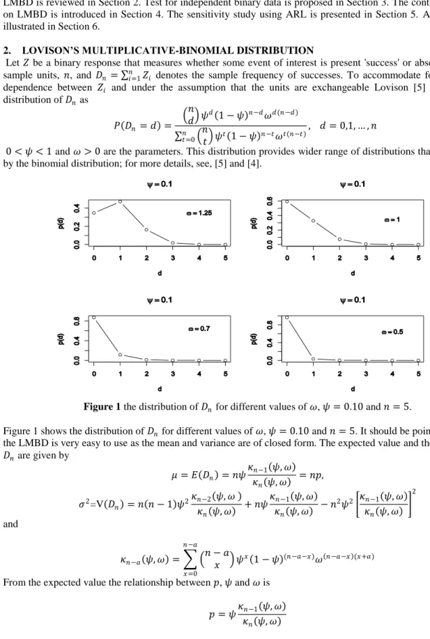
distribution of 𝐷𝑛 as 𝑃 𝐷𝑛 = 𝑑 = 𝑛 𝑑 𝜓𝑑 1 − 𝜓 𝑛−𝑑𝜔𝑑(𝑛−𝑑) 𝑛 𝑡 𝜓𝑡 1 − 𝜓 𝑛−𝑡𝜔𝑡(𝑛−𝑡) 𝑛 𝑡=0 , 𝑑 = 0,1, … , 𝑛
0 < 𝜓 < 1 and 𝜔 > 0 are the parameters. This distribution provides wider range of distributions than are provided by the binomial distribution; for more details, see, [5] and [4].
Figure 1 the distribution of 𝐷𝑛 for different values of 𝜔, 𝜓 = 0.10 and 𝑛 = 5.
Figure 1 shows the distribution of 𝐷𝑛 for different values of 𝜔, 𝜓 = 0.10 and 𝑛 = 5. It should be pointed out that
the LMBD is very easy to use as the mean and variance are of closed form. The expected value and the variance of 𝐷𝑛 are given by 𝜇 = 𝐸 𝐷𝑛 = 𝑛𝜓 𝜅𝑛−1 𝜓, 𝜔 𝜅𝑛 𝜓, 𝜔 = 𝑛𝑝, 𝜎2=V 𝐷 𝑛 = 𝑛 𝑛 − 1 𝜓2 𝜅𝑛−2 𝜓, 𝜔 𝜅𝑛 𝜓, 𝜔 + 𝑛𝜓𝜅𝑛−1 𝜓, 𝜔 𝜅𝑛 𝜓, 𝜔 − 𝑛2𝜓2 𝜅𝑛−1 𝜓, 𝜔 𝜅𝑛 𝜓, 𝜔 2 and 𝜅𝑛−𝑎 𝜓, 𝜔 = 𝑛 − 𝑎 𝑥 𝑛−𝑎 𝑥=0 𝜓𝑥 1 − 𝜓 (𝑛−𝑎−𝑥)𝜔 𝑛−𝑎−𝑥 (𝑥+𝑎)
From the expected value the relationship between 𝑝, 𝜓 and 𝜔 is
𝑝 = 𝜓𝜅𝑛−1 𝜓, 𝜔 𝜅𝑛 𝜓, 𝜔
158
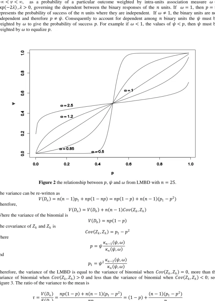
A graph 2 shows this relation. It may explain 𝑝 as a probability of success and 𝜓 = exp 2𝑣 /(1 + exp 2𝑣 ), −∞< 𝑣 <∞, as a probability of a particular outcome weighted by intra-units association measure 𝜔 = exp −2𝜆 , 𝜆 > 0, governing the dependent between the binary responses of the 𝑛 units. If 𝜔 = 1, then 𝑝 = 𝜓 represents the probability of success of the 𝑛 units where they are independent. If 𝜔 ≠ 1, the binary units are not independent and therefore 𝑝 ≠ 𝜓. Consequently to account for dependent among 𝑛 binary units the 𝜓 must be weighted by 𝜔 to give the probability of success 𝑝. For example if 𝜔 < 1, the values of 𝜓 < 𝑝, then 𝜓 must be weighted by 𝜔 to equalize 𝑝.
Figure 2 the relationship between 𝑝, 𝜓 and 𝜔 from LMBD with 𝑛 = 25. The variance can be re-written as
𝑉 𝐷𝑛 = 𝑛 𝑛 − 1 𝑝1+ 𝑛𝑝 1 − 𝑛𝑝 = 𝑛𝑝 1 − 𝑝 + 𝑛 𝑛 − 1 (𝑝1− 𝑝2)
Therefore,
𝑉 𝐷𝑛 = 𝑉 𝐷𝑏 + 𝑛 𝑛 − 1 𝐶𝑜𝑣 𝑍𝑘, 𝑍ℎ
Where the variance of the binomial is
𝑉 𝐷𝑏 = 𝑛𝑝 1 − 𝑝
The covariance of 𝑍𝑘 and 𝑍ℎ is
𝐶𝑜𝑣 𝑍𝑘, 𝑍ℎ = 𝑝1− 𝑝2 where 𝑝 = 𝜓𝜅𝑛−1 𝜓, 𝜔 𝜅𝑛 𝜓, 𝜔 and 𝑝1= 𝜓2 𝜅𝑛−2 𝜓, 𝜔 𝜅𝑛 𝜓, 𝜔
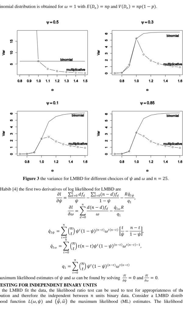
Therefore, the variance of the LMBD is equal to the variance of binomial when 𝐶𝑜𝑣 𝑍𝑘, 𝑍ℎ = 0, more than the
variance of binomial when 𝐶𝑜𝑣 𝑍𝑘, 𝑍ℎ > 0 and less than the variance of binomial when 𝐶𝑜𝑣 𝑍𝑘, 𝑍ℎ < 0; see,
Figure 3. The ratio of the variance to the mean is
𝜏 =𝑉 𝐷𝑛 𝐸 𝐷𝑛 =𝑛𝑝 1 − 𝑝 + 𝑛 𝑛 − 1 (𝑝1− 𝑝 2) 𝑛𝑝 = 1 − 𝑝 + 𝑛 − 1 (𝑝1− 𝑝2) 𝑝
159
The binomial distribution is obtained for 𝜔 = 1 with 𝐸 𝐷𝑛 = 𝑛p and 𝑉 𝐷𝑛 = 𝑛𝑝(1 − 𝑝).
Figure 3 the variance for LMBD for different chocices of 𝜓 and 𝜔 and 𝑛 = 25. From Habib [4] the first two derivatives of log likelihood for LMBD are
𝜕𝑙 𝜕𝜓= 𝑑𝑓𝑑 𝑛 𝑑 =0 𝜓 − (𝑛 − 𝑑)𝑓𝑑 𝑛 𝑑=0 1 − 𝜓 − 𝑅𝑞 1𝜓 𝑞1 , 𝜕𝑙 𝜕𝜔= 𝑑(𝑛 − 𝑑)𝑓𝑑 𝜔 𝑛 𝑑 =0 −𝑞 1𝜔𝑅 𝑞1 where 𝑞 1𝜓 = 𝑛 𝑡 𝑛 𝑡=0 𝜓𝑡 1 − 𝜓 (𝑛−𝑡)𝜔𝑡 𝑛−𝑡 𝑡 𝜓− 𝑛 − 𝑡 1 − 𝜓 , 𝑞 1𝜔= 𝑛 𝑡 𝑛 𝑡=0 𝑡 𝑛 − 𝑡 𝜓𝑡 1 − 𝜓 𝑛−𝑡 𝜔𝑡 𝑛−𝑡 −1, and 𝑞1= 𝑛 𝑡 𝑛 𝑡=0 𝜓𝑡 1 − 𝜓 (𝑛−𝑡)𝜔𝑡 𝑛−𝑡
The maximum likelihood estimates of 𝜓 and 𝜔 can be found by solving 𝜕𝑙
𝜕𝜓 = 0 and
𝜕𝑙 𝜕𝜔 = 0.
3. TESTING FOR INDEPENDENT BINARY UNITS
When the LMBD fit the data, the likelihood ratio test can be used to test for appropriateness of the binomial distribution and therefore the independent between 𝑛 units binary data. Consider a LMBD distribution with likelihood function 𝐿(𝜔, 𝜓) and 𝜓 , 𝜔 the maximum likelihood (ML) estimates. The likelihood ratio test
160
statistic(𝛬) of the hypothesis 𝐻0: 𝜔 = 1 against 𝐻1: 𝜔 ≠ 1 equals 2ln𝐿 between the full model and the reduced
model as
Λ= 2 ln𝐿 𝜓 , 𝜔 −ln𝐿(1, 𝜓 ) = 2 𝑙 𝜓 , 𝜔 − 𝑙(1, 𝜓 )
𝜓 is the ML estimate of the reduced model (binomial model). From Habib [4] the logarithm of likelihood of the sample can be written as
𝑙(𝜓, 𝜔) =log𝑅! + 𝑓𝑑log𝑃 𝑑; 𝜓, 𝜔 − log 𝑓𝑑!
𝑛
𝑑=0 𝑛
𝑑=0
The model under the alternative hypothesis is
𝑙(𝜓 , 𝜔 ) =log𝑅! + 𝑓𝑑log𝑃 𝑑; 𝜓 , 𝜔 − log 𝑓𝑑! 𝑛
𝑑=0 𝑛
𝑑=0
The model under the null hypothesis is
𝑙(𝜓 , 1) =log𝑅! + 𝑓𝑑log𝑃 𝑑; 𝜓 , 1 − log 𝑓𝑑! 𝑛 𝑑=0 𝑛 𝑑=0 Hence, 𝑙 𝜓 , 𝜔 − 𝑙 1, 𝜓 = 𝑓𝑑log𝑃 𝑑; 𝜓 , 𝜔 𝑛 𝑑=0 − 𝑓𝑑log𝑃 𝑑; 𝜓 , 1 𝑛 𝑑=0 Therefore, Λ= 2 𝑓𝑑 log𝑃 𝑑; 𝜓 , 𝜔 −log𝑃 𝑑; 𝜓 , 1 𝑛 𝑑=0
Under the null hypothesis, the test statistic Λ approximately follows chi-square distribution (𝜒2) with one degree of
freedom, see, [8]. See applications below for examples.
4. DEVELOPMENT OF THE CONTROL CHART
When the count data can be modeled by LMBD, the 𝑛𝑝-chart can be obtained as
𝑈𝐶𝐿 = 𝑛𝑝 + 𝑘 𝑛𝑝 1 − 𝑝 + 𝑛 𝑛 − 1 (𝑝1− 𝑝2)
𝐶𝐿 = 𝑛𝑝 and
𝐿𝐶𝐿 = 𝑛𝑝 − 𝑘 𝑛𝑝 1 − 𝑝 + 𝑛 𝑛 − 1 (𝑝1− 𝑝2)
The estimate limits can be obtained using maximum likelihood estimates for 𝜓 and 𝜔. For different 𝜓 and 𝜔 values, the 𝐿𝐶𝐿 would not be positive values especially for near-zero defect process.
a. Upper limit chart
In rare health events and near-zero-defect manufacturing environment, many samples will have no defects. If the LMBD provides a good fit to the data, the upper control limit can be determined by
𝑛 𝑑 𝜓𝑑 1 − 𝜓 𝑛−𝑑𝜔𝑑(𝑛−𝑑) 𝑛 𝑡 𝜓𝑡 1 − 𝜓 𝑛 −𝑡𝜔𝑡(𝑛−𝑡) 𝑛 𝑡=0 = 𝛼 𝑛 𝑑=𝑈𝐶𝐿
where 𝛼 is the probability of false alarm or type 𝐼error.
If we cannot find exact value of UCL that gives 𝛼 we could obtain approximate value of UCL as following: 1. For 𝑈𝐶𝐿1 and 𝑈𝐶𝐿2 find the corresponding 𝛼1, 𝛼2 that include the required 𝛼.
2. The approximate 𝑈𝐶𝐿 = 𝑈𝐶𝐿1+ 𝛼1−𝛼
𝛼2−𝛼1 𝑈𝐶𝐿2− 𝑈𝐶𝐿1 Example
Let 𝛼 = 0.005, 𝑛 = 45, 𝜓 = 0.25 and 𝜔 = .95. The above upper limit does not give the exact 𝛼. The approximated 𝑈𝐶𝐿 is
1. at 𝑈𝐶𝐿1= 7 the value of 𝛼1= 0.0068, and at 𝑈𝐶𝐿2= 8 the value of 𝛼 = 0.0023
161
𝑈𝐶𝐿 ≈ 7 + (0.0068 − 0.005
0.0068 − 0.0023 1 ≈ 7.4
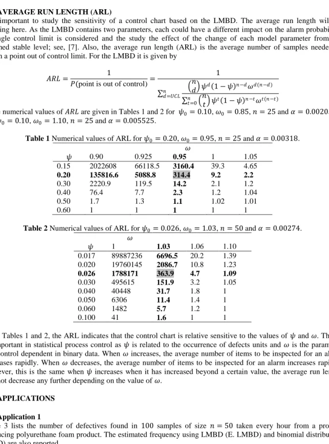
5. AVERAGE RUN LENGTH (ARL)
It is important to study the sensitivity of a control chart based on the LMBD. The average run length will be studying here. As the LMBD contains two parameters, each could have a different impact on the alarm probability. A single control limit is considered and the study the effect of the change of each model parameter from the assumed stable level; see, [7]. Also, the average run length (ARL) is the average number of samples needed to obtain a point out of control limit. For the LMBD it is given by
𝐴𝑅𝐿 = 1
𝑃(point is out of control)=
1 𝑛 𝑑 𝜓𝑑 1 − 𝜓 𝑛−𝑑𝜔𝑑(𝑛−𝑑) 𝑛 𝑡 𝜓𝑡 1 − 𝜓 𝑛−𝑡𝜔𝑡(𝑛−𝑡) 𝑛 𝑡=0 𝑛 𝑑=𝑈𝐶𝐿
Some numerical values of 𝐴𝑅𝐿 are given in Tables 1 and 2 for 𝜓0= 0.10, 𝜔0= 0.85, 𝑛 = 25 and 𝛼 = 0.00205
and 𝜓0= 0.10, 𝜔0= 1.10, 𝑛 = 25 and 𝛼 = 0.005525.
Table 1 Numerical values of ARL for 𝜓0= 0.20, 𝜔0= 0.95, 𝑛 = 25 and 𝛼 = 0.00318.
𝜔 𝜓 0.90 0.925 0.95 1 1.05 0.15 2022608 66118.5 3160.4 39.3 4.65 0.20 135816.6 5088.8 314.4 9.2 2.2 0.30 2220.9 119.5 14.2 2.1 1.2 0.40 76.4 7.7 2.3 1.2 1.04 0.50 1.7 1.3 1.1 1.02 1.01 0.60 1 1 1 1 1
Table 2 Numerical values of ARL for 𝜓0= 0.026, 𝜔0= 1.03, 𝑛 = 50 and 𝛼 = 0.00274.
𝜔 𝜓 1 1.03 1.06 1.10 0.017 89887236 6696.5 20.2 1.39 0.020 19760145 2086.7 10.8 1.23 0.026 1788171 363.9 4.7 1.09 0.030 495615 151.9 3.2 1.05 0.040 40448 31.7 1.8 1 0.050 6306 11.4 1.4 1 0.060 1482 5.7 1.2 1 0.100 41 1.6 1 1
From Tables 1 and 2, the ARL indicates that the control chart is relative sensitive to the values of 𝜓 and 𝜔. This is an important in statistical process control as 𝜓 is related to the occurrence of defects units and 𝜔 is the parameter that control dependent in binary data. When 𝜔 increases, the average number of items to be inspected for an alarm decreases rapidly. When 𝜔 decreases, the average number of items to be inspected for an alarm increases rapidly. However, this is the same when 𝜓 increases when it has increased beyond a certain value, the average run length will not decrease any further depending on the value of 𝜔.
6. APPLICATIONS a. Application 1
Table 3 lists the number of defectives found in 100 samples of size 𝑛 = 50 taken every hour from a process producing polyurethane foam product. The estimated frequency using LMBD (E. LMBD) and binomial distribution (E.BD) are also reported.
162
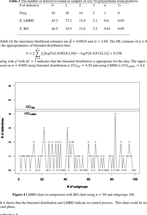
Table 3 The number of defectives found in samples of size 50 polyurethane foam products.
# of defective 0 1 2 3 4 5+
Freq. 45 38 14 2 1 0
E. LMBD 45.3 37.2 13.9 3.1 0.6 0.05 E. BD 46.5 35.9 13.6 3.3 0.61 0.09
From Habib [4] the maximum likelihood estimates are 𝜓 = 0.0024 and 𝜔 = 1.04. The ML estimate of 𝑝 is 0.0152. To test the appropriateness of binomial distribution then
Λ= 2 𝑓𝑑 log𝑃 𝑑; 0.0024,1.04 −log𝑃 𝑑; 0.0152,1 = 0.198
𝑛
𝑑 =0
Comparing with 𝜒2with 𝑑𝑓 = 1 indicates that the binomial distribution is appropriate for the data. The upper control
limit based on 𝛼 = 0.005 using binomial distribution is 𝑈𝐶𝐿𝐵𝐷 = 4.33 and using LMBD is 𝑈𝐶𝐿𝐿𝑀𝐵𝐷 = 4.2.
Figure 4 LMBD chart in comparison with BD chart using 𝑛 = 50 and subgroups 100.
A graph 4 shows that the binomial distribution and LMBD indicate in-control process. This chart could be used in the second phase.
b. Application 2
Table 4 lists the number of defectives found in 200 samples of size 𝑛 = 50 taken every hour from a process producing ballpoint pen cartridges. The estimated frequency using LMBD (E. LMBD) and binomial distribution (E.BD) are also given.
163
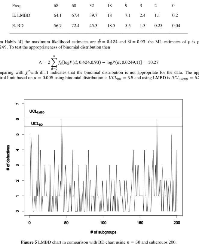
Table 4 The number of defectives found in samples of size 50 ballpoint cartridges.
# of defective 0 1 2 3 4 5 6 7+
Freq. 68 68 32 18 9 3 2 0
E. LMBD 64.1 67.4 39.7 18 7.1 2.4 1.1 0.2
E. BD 56.7 72.4 45.3 18.5 5.5 1.3 0.25 0.04
From Habib [4] the maximum likelihood estimates are 𝜓 = 0.424 and 𝜔 = 0.93. the ML estimates of 𝑝 is 𝑝 = 0.0249. To test the appropriateness of binomial distribution then
Λ= 2 𝑓𝑑 log𝑃 𝑑; 0.424,0.93 −log𝑃 𝑑; 0.0249,1 = 10.27
𝑛
𝑑 =0
Comparing with 𝜒2with df=1 indicates that the binomial distribution is not appropriate for the data. The upper
control limit based on 𝛼 = 0.005 using binomial distribution is 𝑈𝐶𝐿𝐵𝐷 = 5.5 and using LMBD is 𝑈𝐶𝐿𝐿𝑀𝐵𝐷= 6.2.
Figure 5 LMBD chart in comparison with BD chart using 𝑛 = 50 and subgroups 200.
A graph 5 shows that the binomial distribution indicates out-of-control process. On the other hand the LMBD chart shows in-control process and fit the data 𝜒𝐿𝑀𝐵𝐷2 = 2.68 < 𝜒2,0.052 = 5.99. This may indicate that the chart based on
164 7. CONCLUSION
When analyzing defect data with correlated binary data, the chart based on binomial distribution has drawback in producing many false alarms which results in high cost of inspection and frequent stopping of the manufacturing processes. LMBD instead of binomial distribution is suitable in this situation where more appropriate upper control limit can be derived. Average run length approach is used to evaluate the performance of the proposed chart. The main advantage of this chart is that if the binary data are independent the LMBD reduces to binomial distribution. REFERENCES
[1]. Altham, P. (1978) Two generalizations of the binomial distribution. Applied Statistics, 27, 162-167. [2]. Cox, D.R. (1972) The analysis of multivariate binary data. Applied Statistics, 21, 113-120.
[3]. Elamir, E and Seheult, A. (2001) Control charts based on linear combinations of order statistics. Journal of Applied Statistics, 28, 457-468.
[4]. Habib, E (2010) Estimation of log-linear-binomial distribution with applications. Journal of Probability and Statistics, 10, 7-20.
[5]. Lovison, G. (1998) An alternative representation of Altham's multiplicative-binomial distribution. Statistics & Probability Letters, 36, 415-420.
[6]. Montgomery, D.C. (2005) Introduction to Statistical Quality Control. 5th e,, Wiley, New York.
[7]. Ott, E.R., Schilling, E.G. and Neubauer, D.V. (2005) Process quality control: troubleshooting and interpretation of data. 4th ed. Quality Press, ASQ.
[8]. Severini, T.A. (2000). Likelihood methods in statistics. (1st Ed.), Oxford University Press.
[9]. Sim, C.H. and Lim, M.H. (2008) Attribute charts for zero-inflated processes. Communications in Statistics:
Simulation and Computation, 34, 201-209.
[10]. Woodal, W.H. (2006) The use of control charts in health-care and public-health surveillance. Journal of
Quality Technology, 38, 88-103.
[11]. Xie, M., He, B. and Goh, T.N. (2001) Zero-inflated Poisson model in statistical process control.