Assessments of Some Simultaneous Equation Estimation Techniques with Normally and Uniformly Distributed Exogenous Variables

(1)

http://dx.doi.org/10.4236/am.2015.611167

Assessments of Some Simultaneous

Equation Estimation Techniques with

Normally and Uniformly Distributed

Exogenous Variables

O. O. Alabi

1

, B. A. Oyejola

2

1_{Department of Statistics, Federal University of Technology, Akure, Nigeria} 2_{Department of Statistics, University of Ilorin, Ilorin, Nigeria}

Email: [email protected], [email protected], [email protected]

Received 8 September 2015; accepted 24 October 2015; published 27 October 2015

This work is licensed under the Creative Commons Attribution International License (CC BY).

http://creativecommons.org/licenses/by/4.0/

Abstract

In each equation of simultaneous Equation model, the exogenous variables need to satisfy all the basic assumptions of linear regression model and be non-negative especially in econometric stu-dies. This study examines the performances of the Ordinary Least Square (OLS), Two Stage Least Square (2SLS), Three Stage Least Square (3SLS) and Full Information Maximum Likelihood (FIML) Estimators of simultaneous equation model with both normally and uniformly distributed ex-ogenous variables under different identification status of simultaneous equation model when there is no correlation of any form in the model. Four structural equation models were formed such that the first and third are exact identified while the second and fourth are over identified equations. Monte Carlo experiments conducted 5000 times at different levels of sample size (n = 10, 20, 30, 50, 100, 250 and 500) were used as criteria to compare the estimators. Result shows that OLS estimator is best in the exact identified equation except with normally distributed ex-ogenous variables when n≥100. At these instances, 2SLS estimator is best. In over identified eq-uations, the 2SLS estimator is best except with normally distributed exogenous variables when the sample size is small and large, n=10 and n≥250; and with uniformly distributed exogenous variables when n is very large, n=500, the best estimator is either OLS or FIML or 3SLS.

Keywords

(2)

1. Introduction

A simultaneous equation system is a regression equation system where two types of variables (the endogenous, the predetermined or exogenous variable) appear with disturbance terms. [1] defined simultaneous equation as the process of modeling more than one equation at a time; a multi-equation modeling. It is proposed to solve the problem of correlation.

In a multi-equation model, the dependent variable Y appears as endogenous variable in one equation and as explanatory variable in another equation of the model. The X variable appears as the explanatory variable in the equations. This creates problems of equation identification, multicollinearity and choice of estimation tech-niques among others.

Identification problem which creates estimation problems has the same features with multicollinearity [2]. Correlation between the pairs of exogenous or independent variables is an important problem in econometrics especially in single equation estimation. The impact of multicollinearity is less serious when attention is focused on predicting or forecasting values of the endogenous variables than when the analyst is interested in estimating the parameters [3].

Econometric variables are often non-negative and can exhibit violation against the normality assumption of classical models which inevitably influences the performances of the estimation techniques. This study therefore examines the performances of four (4) common estimation techniques namely; Ordinary Least squares (OLS), Two-stage Least squares (2SLS), Three-stage Least squares (3SLS) and Full Information Maximum Likelihood Estimators under both normally and uniformly distributed exogenous variables for different equation identifica-tion status. Here it is assumed that there is no form of correlaidentifica-tion in the simultaneous equaidentifica-tion model.

Most economic data are often positive [4] and correlated [5]. However, various works done in the recent time especially on correlation studies on simultaneous equation model have being with normally distributed exogen-ous variables, exhibiting both positive and negative values [6] [7].

2. Methodology

The methodology followed in this research work is as follows:

The Model and Its Description

Consider the simultaneous Equation model of the for

1 12 2 13 3 14 4 14 4 1

2 23 3t 21 1 23 3 2

3 31 1 34 4 31 1t 32 2 3

4 41 1 42 42 42 2t 4

(i)

y (ii)

(iii) (iv)

t t t t t t

t t t t

t t t t t

t t t

y y y y x u

y x x u

y y y x x u

y y y x u

β β β γ

β γ γ

β β γ γ

β β γ

= + + + +

= + + +

= + + + +

= + + +

(1)

where y_it is an endogenous variable, i=1, 2, 3, 4_; x₁t,x₂t,x₃t and x4t are the exogenous variables

( )

1

2

3

4

~ 0,

t

t u

u N u u    

  _Σ

       

where t=1, 2, 3,,n and β β β β β β β β γ γ γ γ γ₁₂, ₁₃, ₁₄, ₂₃, ₃₁, ₃₄, ₄₁, ₄₂, ₁₄, ₂₁, ₂₃, ₃₁, ₃₂ and γ₄₂ are the structural pa-rameters of the model. Equations (i) and (iii) are exactly identified while Equations (ii) and (iv) were over iden-tified by both order and rank condition.

For the simulation study, Equation (1) was expressed as follows:

1 12 2 13 3 14 4 1 2 3 14 4 1

31 1 2 3 34 4 31 1t 32 2 3 4 3

41 1 42 2 3 4 1 42 2t 3 4 4

0 0 0 (i)

0 0 0 (iii)

0 0 0 0

t t t t t t t t t

t t t t t t t t

y y y y x x x x u

β β β γ

β β γ γ

β β γ

− − − + + + − =

− + + − − − + + =

− − + + + − + + = (iv)

(4)

This can be written in matrix form as:

t t t

y x u

(3)

where

12 13 14

23

31 34

41 42

1

0 1 0

0 1

β β β

β β β β β β − − −    ₋    = − −  ₋ ₋    , 14 21 23 31 32 42

0 0 0

0 0

0 0 0

γ γ γ γ γ γ −   ₋ ₋    Γ = − −   ₋    , 1 2 3 4 t y y y y y       =       , 1 2 3 4 t x x x x x         =         and 1 2 3 4 t u u u u u       =      

Now, from (5),

1 1 1

t t t

y x u

β β− ₌β−_{Γ =}β−

1 1

t t t

y =β−Γ +x β−u (6)

Equation (6) was used to generate the endogenous variables by taking the true value of the parameters as:

12 13 14

23

31 34

41 42

1

0 1 0

0 1

β β β

β β β β β β − − −    ₋    = − −    − −   14 21 23 31 32 42

0 0 0

0 0

0 0 0

γ γ γ γ γ γ −   ₋ ₋    Γ = − −   ₋   

Monte Carlo experiments were performed 5000 times for seven sample sizes (n = 10, 20, 30, 50, 100, 250 and 500) when there is no correlation of any form among exogenous variables and the error terms. The two forms of exogenous variables are generated to follow normal and uniform distribution.

3. Data Generation of Exogenous Variables

The generation was done as follows:

1) Normally Distributed Exogenous Variables

The exogenous were generated to be normal with mean zero and variance unity i.e. xi ~N

( )

0,1 ,i=1, 2, 3, 4

and

ρ

_ij <1 is the value of correlation between the two variables i and j, [8]. In this study,

12 13 14 23 24 34 0

ρ =ρ =ρ =ρ =ρ =ρ = =ρ , was adopted as a situation with no forms of any correlation between the exogenous variables.

2)Correlated Uniformly Distributed Variables

Using the generated normally distributed exogenous variables above, Xi ~N

( )

0,1 , I = 1, 2, 3, 4; we fur-ther utilize the properties of random variables that cumulative distribution function of normal distribution pro-duces U(0, 1) without affecting the correlation among the variables to generate correlated uniformly distributed exogenous variables, Xi ~U

( )

0,1 , I = 1, 2, 3, 4; [9].

3) Generation of Correlated Error Terms

Equation provided by [8] was modified when the mean of the error terms are zero and variance is unit (1). Also,

λ

ij <1 is the value of correlation between the two error terms i and j. In this study,

12 13 14 23 24 34 0

(4)

4) Method of Generating the Data of Endogenous Variables

Equation (6) was used to generate the endogenous variables by taking the true value of the parameters as:

12 13 14

23

31 34

41 42

1 1 3.2 0.2 1.2 0 0 0 0.8

0 1 0 0 1 3.8 0 3.0 0 1.3 0

0 1 1.6 0 1 1.0 1.5 0.6 0 0

0 1 2.8 2.2 0 1 0 2.6 0 0

β β β

β β

− − − − − − −

     

 ₋   ₋  ₋ ₋ 

     

= = =

− −  − −  − − 

₋ ₋     

− − −

   

 

5) Criteria Used for Assessment of the Estimators

To assess the performance of the estimators, the finite properties were used (Bias, Absolute bias, Variance and Mean Square Error):

Mathematically, MSE is the addition of the Bias squared to the variance. For any estimator

θ

ˆ_ij of

θ

_ij in model (1),

1

ˆ R ˆ

ij ijl

l R

θ

=

∑

, l=1, 2,,R

where R = 5000

( )

ˆ ˆ

BIAS

θ

_ij =

θ θ

_ij− _ij

( )

1

ˆ ˆ

ABSBIAS ,

R

ij ijl ij

l R

θ

=

∑

−

as a measure of dispersion.

( )

(

)

2

1

ˆ ˆ

MSE

R

ij ijl ij

l R

θ

=

∑

−

( )

2

ˆ ˆ ˆ

Var θ_ij =MSE θ_ij − Bias θ_ij _

In this paper, θˆ is used to represent any of the parameters in (1).

4. Results and Discussion

4.1. Performance of the Estimator Based on the Bias Criterion

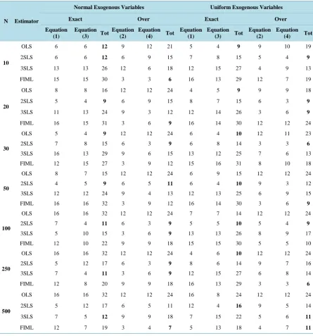
The performances of the estimators was examined, ranked and summed over all the parameters in each equation, having examined and summed the rank of the bias of each parameter over all the parameters in each equation the outcome is given in Table 1.

The preferred estimators for different identification status differ. The preferred estimators are also slightly af-fected by the two exogenous variables.

In the exact identified equation with normally distributed exogenous variables, OLS or 2SLS or both are gen-erally preferred except for very large samples sizes

(

n≥250

)

. At this instance, 3SLS is preferred. Also, with uniformly distributed exogenous variables, OLS or 2SLS estimators are generally preferred.

In the over identified equation with normally distributed exogenous variable, 2SLS estimator is generally preferred except when n≤20_{and when} n=500. At these instances, FIML estimator is preferred.

Also, with uniformly distributed exogenous variable 2SLS estimator is generally preferred except at very large sample sizes when n=50 and when n=250. At these instances, the FIML estimator is preferred.

4.2. Performances of the Estimators Based on Absolute Bias Criterion

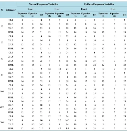
The performances of the estimators was examined, ranked and summed over all the parameters in each equation, having examined and summed the rank of absolute bias of each parameter over all the parameters in each equa-tion the outcome is given in Table 3.

From Table 3, at each level of sample size the sum rank were further added over the equations and preferred estimator under both exact and over identification model with the two exogenous variables were bolded.Table 4

gives the summary of the findings as follows:

(5)

[image:5.595.89.535.100.578.2]

Table 1. Summary of the total ranks of the parameter based on bias criterion when there is no correlation.

N Estimator

Normal Exogenous Variables Uniform Exogenous Variables

Exact Over Exact Over

Equation (1)

Equation (3) Tot

Equation (4) Tot

Equation (3) Tot

Equation (4) Tot

10

OLS 6 6 12 9 12 21 5 4 9 9 10 19 2SLS 6 6 12 6 9 15 7 8 15 5 4 9

3SLS 13 13 26 12 6 18 12 15 27 4 9 13 FIML 15 15 30 3 3 6 16 13 29 12 7 19

20

OLS 8 8 16 12 12 24 4 5 9 9 9 18 2SLS 5 4 9 6 9 15 8 7 15 6 3 9

3SLS 11 13 24 9 3 12 12 14 26 3 6 9

FIML 16 15 31 3 6 9 16 14 30 12 12 24

30

OLS 5 4 9 12 12 24 6 4 10 12 11 23 2SLS 7 8 15 6 3 9 6 8 14 3 3 6

3SLS 16 13 29 9 6 15 13 12 25 7 6 13 FIML 12 15 27 3 9 12 15 16 31 8 10 18

50

OLS 8 7 15 12 12 24 6 9 15 12 12 24 2SLS 4 5 9 6 5 11 6 4 10 9 3 12 3SLS 12 12 24 9 4 13 12 13 25 6 9 15 FIML 16 16 32 3 9 12 16 14 30 3 6 9

100

OLS 16 16 32 12 12 24 7 7 14 12 12 24 2SLS 7 4 11 6 3 9 5 5 10 5 4 9

3SLS 5 10 15 3 6 9 13 13 26 8 9 17 FIML 12 10 22 9 9 18 15 15 30 5 5 10

250

OLS 16 16 32 12 12 24 4 6 10 12 12 24 2SLS 5 12 17 6 3 9 8 6 14 9 7 16 3SLS 7 4 11 3 6 9 12 15 27 6 8 14 FIML 12 8 20 9 9 18 16 13 29 3 3 6

500

OLS 16 16 32 12 12 24 16 8 24 12 12 24 2SLS 5 12 17 6 5 11 12 4 16 9 5 14 3SLS 7 5 12 9 9 18 7 15 22 5 6 11

FIML 12 7 19 3 4 7 5 13 18 4 7 11

Source: Computed from simulated results of bias criterion.

by the two exogenous variables. In the exact identified equation with normally distributed exogenous variables under the absolute bias criterion the OLS estimators is preferred when n≤50 and the 2SLS estimator when

50 n .

With uniformly distributed exogenous variables the OLS estimator is generally preferred.

In the over identified equation with normally distributed exogenous variables under the absolute bias criterion, the OLS estimator is preferred when the sample size is small n=10; 2SLS estimator when 20≤ ≤n 50; and FIML when n50.

(6)

4.3. Performances of the Estimators Based on Variance Criterion

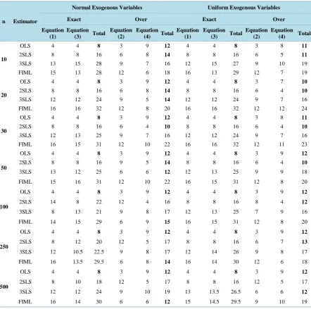
The performances of the estimators was examined, ranked and summed over all the parameters in each equation, having examined and summed the rank of the variance of each parameter over all the parameters in each equa-tion the outcome is given in Table 5.

FromTable 5, at each level of sample size the sum rank were further added over the equations, and preferred estimator under both exact and over identification model with the two exogenous variables were bolded. Table 6

gives the summary of the findings as follows:

From Table 6, the following are observed about the preferred estimators under the variance criterion.

The preferred estimators differ in term of identification status. The preferred estimators are slightly affected by the two exogenous variables.

In the exact identified equation, the OLS estimator is generally preferred in all the sample sizes for both ex-ogenous variables. In the over identified equation with normally distributed exex-ogenous variables, OLS or 2SLS estimator are preferred when n≤50; but for n50, the OLS or FIML estimator are preferred. With un-iformly distributed exogenous variables the OLS or 2SLS estimators are generally preferred. Moreover, the 3SLS estimator replaces the 2SLS when the sample sizes is very large, n=500.

4.4. Performances of the Estimators Based on Mean Squared Error Criterion

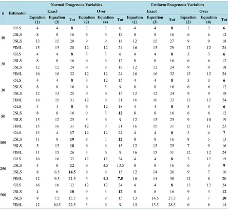
The performances of the estimators was examined, ranked and summed over all the parameters in each equation, having examined and summed the rank of the mean squared error of each parameter over all the parameters in each equation the outcome is given inTable 8.

From Table 8the following are observed about the preferred estimators under the mean squared error crite-rion.

The preferred estimators differ in term of identification status. The preferred estimators are slightly affected by the two exogenous variables. In the exact identified equation with normally distributed exogenous variables, the OLS estimator is generally preferred except when the sample size is large n≥250. At these instances 2SLS is generally preferred. With uniformly distributed exogenous variables, the OLS estimator is generally preferred. In the over identified equation with normally distributed exogenous variables, the OLS estimators is preferred when n≤20; 2SLS when 30≤ ≤n 100, and FIML when n≥100. With uniformly distributed exogenous va-riables the OLS estimators is preferred except when the sample size is large, n≥250. At these instances, the 2SLS estimator is generally preferred. The performance of the preferred estimators is more stable with uniform-ly distributed exogenous variables than the normaluniform-ly distributed exogenous variables.

4.5. Performances of the Estimators Based on All the Criteria

FromTable 10, the following are observed about the preferred estimators under the overall criteria.

The preferred estimators differ in term of identification status. The preferred estimators are slightly affected by the two exogenous variables.

In the exact identified equation with normally distributed exogenous variables the OLS estimator is general-ly preferred except when the sample size is large when n≥100. At these instances, 2SLS is preferred. With uniformly distributed exogenous variable, the OLS estimator is preferred for all sample sizes.

In the over identified equation with normally exogenous variables the OLS estimators is preferred when the samples sizes is small n=10; 2SLS when 20≤ ≤n 30, and n=100; 3SLS when n=50 and FIML estima-tor with n≥250_.

With uniformly distributed exogenous variable, the 2SLS estimator is preferred except when the sample sizes is large n=500. At this instance the 3SLS estimator is preferred.

From Table 1, at each level of sample size the sum rank were further added over the equations, and preferred estimator under both exact and over identification model with the two exogenous variables were bolded. Table 2

gives the summary of the preferred estimators.

From Table 3, at each level of sample size, the sum rank were further added over the equations, and preferred estimator under both exact and over identification model with the two exogenous variables were bolded. Table 4

(7)

[image:7.595.92.537.98.218.2]

Table 2. Summary of the preferred estimators based on bias criterion.

Sample sizes Normal Exogenous Variables Uniform Exogenous Variables

10 OLS\2SLS FIML OLS 2SLS 20 2SLS FIML OLS 2SLS\3SLS 30 OLS 2SLS OLS 2SLS 50 2SLS 2SLS 2SLS FIML 100 2SLS 2SLS\3SLS 2SLS 2SLS 250 3SLS 2SLS\3SLS OLS FIML 500 3SLS FIML 2SLS 2SLS\FIML

Source: Table 1.

Table 3. Performances of the estimator based on absolute bias criterion.

N Estimator

Equation (3) Tot

Equation (4) Tot

Equation (3) Tot

Equation (4) Tot

10

OLS 4 4 8 3 3 6 4 4 8 4 3 7

2SLS 8 8 16 6 6 12 8 8 16 5 6 11 3SLS 12 13 25 9 9 18 12 14 26 9 9 18 FIML 16 15 31 12 12 24 16 14 30 12 12 24

20

OLS 4 4 8 10 12 22 4 4 8 5 6 11

2SLS 8 8 16 3 3 6 8 8 16 4 4 8

3SLS 12 12 24 6 6 12 12 12 24 9 8 17 FIML 16 16 32 11 9 20 16 16 32 12 12 24

30

OLS 4 4 8 12 12 24 4 4 8 9 5 14 2SLS 8 8 16 3 3 6 8 8 16 3 4 7

3SLS 12 13 25 9 6 15 12 12 24 6 9 15 FIML 16 15 31 6 9 15 16 16 32 12 12 24

50

OLS 5 4 9 12 12 24 4 4 8 6 9 15 2SLS 7 8 15 6 3 9 8 8 16 3 4 7

3SLS 12 12 24 3 6 9 12 13 25 9 7 16 FIML 16 16 32 9 9 18 16 15 31 12 10 22

100

OLS 16 10 26 12 12 24 4 4 8 10 11 21 2SLS 4 4 8 9 3 12 8 8 16 5 3 8 3SLS 8 12 20 6 9 15 12 13 25 4 7 11 FIML 12 14 26 3 6 9 16 15 31 11 9 20

250

OLS 16 16 32 12 12 24 4 4 8 12 12 24 2SLS 4 6 10 9 5 14 8 8 16 3 3 6 3SLS 8 8 16 6 9 15 12 13 25 6 8 14 FIML 12 10 22 3 4 7 16 15 31 9 7 16

500

OLS 16 16 32 12 12 24 10 5 15 12 12 24 2SLS 4 6 10 9 5.5 14.5 6 7 13 9 3 12 3SLS 8 8.5 16.5 6 8 14 10 14 24 5 8 13 FIML 12 9.5 21.5 3 4.5 7.5 14 14 28 4 7 11

[image:7.595.91.534.251.707.2]

(8)

[image:8.595.89.536.98.231.2]

Table 4. Summary of the preferred estimators based on absolute bias criterion.

10 OLS OLS OLS 2SLS

20 OLS 2SLS OLS 2SLS 30 OLS 2SLS OLS 2SLS 50 OLS 2SLS\3SLS OLS 2SLS 100 2SLS FIML OLS 2SLS 250 2SLS FIML OLS 2SLS 500 2SLS FIML 2SLS\OLS FIML\2SLS\3SLS

Source: Table 3.

Table 5. Performances of the estimators based on variance criterion.

n Estimator

Equation (3) Total

10

OLS 4 4 8 3 9 12 4 4 8 3 8 11

2SLS 8 8 16 6 8 14 8 8 16 6 5 11

3SLS 13 15 28 9 7 16 12 15 27 9 10 19 FIML 15 13 28 12 6 18 16 13 29 12 7 19

20

OLS 4 4 8 3 9 12 4 4 8 3 7 10

2SLS 8 8 16 6 8 14 8 8 16 6 4 10

3SLS 12 12 24 9 5 14 12 12 24 9 7 16 FIML 16 16 32 12 8 20 16 16 32 12 12 24

30

OLS 4 4 8 3 9 12 4 4 8 3 8 11

2SLS 8 8 16 6 4 10 8 8 16 6 4 10

3SLS 12 13 25 9 7 16 12 12 24 9 7 16 FIML 16 15 31 12 10 22 16 16 32 12 11 23

50

OLS 4 4 8 3 9 12 4 4 8 3 9 12

2SLS 8 8 16 9 5 14 8 8 16 6 4 10

3SLS 13 12 25 6 6 12 12 13 25 9 9 18 FIML 15 16 31 12 10 22 16 15 31 12 8 20

100

OLS 4 4 8 3 9 12 4 4 8 3 9 12

2SLS 14 8 22 12 4 16 8 8 16 8 4 12

3SLS 8 13 21 9 8 17 12 13 25 7 9 16 FIML 14 15 29 6 9 15 16 15 31 12 8 20

250

OLS 4 4 8 3 9 12 4 4 8 3 9 12

2SLS 8 12 20 12 5 17 8 8 16 6 7 13

3SLS 12 10.5 22.5 9 8 17 12 14 26 9 8 17 FIML 16 13.5 29.5 6 8 14 16 14 30 12 6 18

500

OLS 4 4 8 3 9 12 4 4 8 3 9 12

2SLS 8 10 18 12 5 17 8 8 16 12 5 17 3SLS 12 12 24 9 10 19 13 13.5 26.5 6 6 12

FIML 16 14 30 6 6 12 15 14.5 29.5 9 10 19

[image:8.595.92.535.268.707.2]

(9)

[image:9.595.91.538.145.268.2]

estimators under both exact and over identification model with the two exogenous variables were made bold.

Table 6 gives the summary of the preferred estimators.

FromTable 7, at each level of sample size the sum rank were further added over the equations and preferred

Table 6. Summary of the preferred estimators under variance criterion.

10 OLS OLS\2SLS OLS OLS\2SLS 20 OLS OLS\2SLS\3SLS OLS OLS\2SLS 30 OLS 2SLS\OLS OLS 2SLS\OLS 50 OLS OLS\2SLS\3SLS OLS 2SLS\OLS 100 OLS OLS\FIML OLS OLS\2SLS 250 OLS OLS\FIML OLS OLS\2SLS 500 OLS OLS\FIML OLS OLS\3SLS

[image:9.595.90.535.301.708.2]

Table 7. Performances of the estimators based on mean squared error criterion.

n Estimator

Equation (3) Tot

Equation (4) Tot

Equation (3) Tot

Equation (4) Tot

10

OLS 4 4 8 3 3 6 4 4 8 3 3 6

2SLS 8 8 16 6 6 12 8 8 16 6 6 12 3SLS 13 15 28 9 9 18 12 15 27 9 9 18 FIML 15 13 28 12 12 24 16 13 29 12 12 24

20

OLS 4 4 8 3 3 6 4 4 8 3 3 6

2SLS 8 8 16 6 6 12 8 8 16 6 6 12 3SLS 12 12 24 9 9 18 12 12 24 9 9 18 FIML 16 16 32 12 12 24 16 16 32 12 12 24

30

OLS 4 4 8 3 12 15 4 4 8 3 3 6

2SLS 8 8 16 6 3 9 8 8 16 6 6 12 3SLS 12 13 25 9 6 15 12 12 24 9 9 18 FIML 16 15 31 12 9 21 16 16 32 12 12 24

50

OLS 4 4 8 6 12 18 4 4 8 3 3 6

2SLS 8 8 16 9 3 12 8 8 16 6 6 12 3SLS 13 12 25 3 6 9 12 13 25 9 10 19 FIML 15 16 31 12 9 21 16 15 31 12 11 23

100

OLS 13 4 17 12 12 24 4 4 8 3 4 7

2SLS 11 8 19 9 3 12 8 8 16 8 5 13 3SLS 5 13 18 6 9 15 12 13 25 7 9 16 FIML 11 15 26 3 6 9 16 15 31 12 12 24

250

OLS 16 16 32 12 12 24 4 4 8 3 12 15 2SLS 4 8 12 9 4.5 13.5 8 8 16 6 3 9

3SLS 8 6.5 14.5 6 9 15 12 14 26 9 7 16 FIML 12 9.5 21.5 3 4.5 7.5 16 14 30 12 8 20

500

OLS 16 16 32 12 12 24 4 4 8 12 12 24 2SLS 4 6 10 9 3 12 8 8 16 9 3 12

3SLS 8 7.5 15.5 6 9 15 13 14.5 27.5 3 7 10

FIML 12 10.5 22.5 3 6 9 15 13.5 28.5 6 8 14

(10)

estimator under both exact and over identification model with the two exogenous variables were bolded.Table 8

4.6. Overall Examination of the Model Parameters

The overall summary of the performances of the estimators having examined and obtained by adding the total ranks over all the criteria is given inTable 9.

FromTable 9, at each level of sample size the sum of the rank were further added over all the criteria and preferred estimator under both exact and over identification model with the two exogenous variables were bolded. Table 10 gives the summary of the preferred estimators.

Table 8. Summary of the preferred estimators when there is no correlation under mean squared error criterion.

10 OLS OLS OLS OLS

20 OLS OLS OLS OLS

30 OLS 2SLS OLS OLS

50 OLS 3SLS\2SLS OLS OLS 100 OLS\2SLS\3SLS 2SLS\FIML OLS OLS 250 2SLS\3SLS FIML OLS 2SLS 500 2SLS FIML\2SLS OLS 3SLS\2SLS

Table 9. Overall performances of the estimators based on all criteria.

N Estimator Normal Uniform

EXACT OVER EXACT OVER

10

OLS 36 45 33 43

2SLS 60 53 63 43

3SLS 107 70 107 68 FIML 117 72 117 86

20

OLS 40 64 33 45

2SLS 57 47 63 39

3SLS 96 56 98 60 FIML 127 73 126 96

30

OLS 33 75 34 54

2SLS 63 34 62 35

3SLS 104 61 97 62 FIML 120 70 127 89

50

OLS 40 78 39 57

2SLS 56 46 58 41

3SLS 98 43 100 68 FIML 126 73 123 74

100

OLS 83 84 38 64

2SLS 60 49 58 42

3SLS 74 56 101 60 FIML 103 51 123 74

250

OLS 104 84 34 75 2SLS 59 53.5 62 44

3SLS 64 56 104 61 FIML 93 46.5 120 60

500

OLS 104 84 55 84 2SLS 55 54.5 61 55 3SLS 68 66 100 46

FIML 93 35.5 104 55

(11)

[image:11.595.89.540.97.244.2]

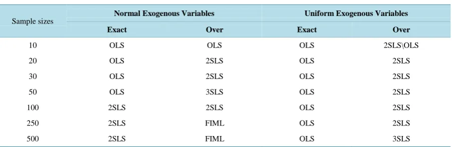
Table 10. Overall summary of the best estimators on the basis of all criteria.

Sample sizes

10 OLS OLS OLS 2SLS\OLS 20 OLS 2SLS OLS 2SLS 30 OLS 2SLS OLS 2SLS 50 OLS 3SLS OLS 2SLS 100 2SLS 2SLS OLS 2SLS 250 2SLS FIML OLS 2SLS 500 2SLS FIML OLS 3SLS

Source: Table 4and Table 9.

5. Conclusions

The performances of the estimators are affected by the distribution of the exogenous variables. The best estima-tors are more stable over the levels of sample size with uniformly distributed exogenous variables than the nor-mally distributed exogenous variables.

In exact identified equation with normally distributed exogenous variables the following were observed. For low sample sizes, OLS is the best performed estimator. In medium sample sizes, OLS or 2SLS is the best performed estimator and 2SLS estimator is the best performed in the large sample sizes. Whereas with uniform-ly distributed exogenous variables, OLS is the best performed estimator in the entire sample sizes category.

In over identified equation with normally distributed exogenous variables, the following are observed.

For low sample sizes, OLS or 2SLS is the best performed estimator, in medium sample sizes 2SLS\3SLS is the best performed estimator and FIML estimator performed best in the large sample sizes. Whereas with un-iformly distributed exogenous variables, 2SLS is the best in low and medium sample sizes category, but 2SLS/ 3SLS estimator is the best in large sample sizes category.

Hence, when there is no correlation of any form in the model the performances of the estimators are affected by the distribution of the exogenous variables in simultaneous equation models.

References

[1] Schmidt, J.S. (2005) Econometrics. McGraw-Hill International Edition.

[2] Koutsoyainnis, A. (1977) Theory of Econometrics. 2nd Edition, Palgrave Publishers Ltd., New York.

[3] Odunta, E.A. (2004) A Monte Carlo Study of the Problem of Multicollinearity in a Simultaneous Equation Model. Unpulished Ph.D. Thesis, Department of Statistics University of Ibadan, Ibadan.

[4] Kmenta, J. and Gilberet, R.F. (1967) Small Sample Properties of Alternative Estimators of Seemingly Unrelated Re-gression. Journal of the American Statistical Association, 63, 1180-1200.

http://dx.doi.org/10.1080/01621459.1968.10480919

[5] Chatterjee, S. and Ali, S.H. (2012) Regression Analysis by Example. 5th Edition, John Wiley and Sons, Hoboken.

[6] Johnson, T.L., Ayinde, K. and Oyejola, B.A. (2010) Effect of Correlations and Equation Identification Status on Esti-mators of a System of Simultaneous Equation Model. Electronic Journal of Applied Statistical Analysis EJASA, 3, 115-125. http://siba-ese.unile.it/index.php/ejasa/index

[7] Ayinde, K., Johnson, T.L. and Oyejola, B.A. (2011) Effect of Equation Identification Status and Correlation between Error Terms on Estimators of System of a Simultaneous Equation Model. American Journal of Scientific and Industrial Research, 2, 184-190. http://dx.doi.org/10.5251/ajsir.2011.2.2.184.190

[8] Ayinde, K. (2007) Equation to Generate Normal Variates with Desired Intercorrelations Matrix. International Journal of Statistics and System, 2, 99-111.