SOLVING ECONOMIC DISPATCH PROBLEM USING PARTICLE SWARM OPTIMIZATION BY AN EVOLUTIONARY TECHNIQUE FOR INITIALIZING PARTICLES

747

ANALYSIS INFLUENCE FACTORS ON LINEAR CCD’S

INTERNAL PARAMETER CALIBRATION

ZHIYONG LEI,ZHENXING ZHU,ZEMIN WANG

School of Electronic Information Engineering, Xi’an Technological University, Xi’an 710032, Shanxi,

China

ABSTRACT

In order to improve the measurement accuracy of the linear CCD in the intersection of vertical target measurement system, the calibration model of linear CCD’s internal parameters is established and the various factors that affect the accuracy in the calibration process are analyzed. Making use of the linear CCD imaging optical principle, the optical center and the effective focal length are calibrated by using upright and inverted mirror state theory and N-style array streak model respectively. It can be proved through theoretical analysis and argument that the method can effectively reduce the impact of the factors as real object height to calibration accuracy and obtain the high precision calibration results which are satisfied the application indicators of linear CCD in the intersection of vertical target measurement system. It can be known from the experimental data that the optical canter calibration accuracy is less than 0.29 pixels and the focal length is less than 2.5‰.

Keywords: Linear CCD, Influence Factors, Calibration, Upright and Inverted Mirror State, N-style Array

Steak Model.

1. INTRODUCTION

The intersection of vertical target measurement system is a very common weapon firing accuracy measurement system in field of modern military[1]. Linear CCD is widely used in these measurement systems with not only its wide angle of view but

also the great advantage in high-speed

measurement.

The calibration of the model parameters of linear CCD has a direct impact on the measurement accuracy of the intersection measuring system. The existing linear CCD calibration methods are improvement of classic plane camera calibration methods like radial constraint calibration[2] or the 2D planar targets calibration[3]. These methods are ported into a two-dimensional flat space to be calibrated from three-dimensional space through some certain conversion relation. However, these kinds of calibration methods ignore the results of a nonlinear lens distortion parameters caused by distortion of camera lens[4-6]. Besides, under the situation of failing to make sure the view of linear CCD during calibration, these methods may produce calculation errors on the actual physical height, and then affect the calibration accuracy. In the mathematical model calibrated by internal parameters of linear CCD, the accuracy of

parameter measurement will impact the results of calibration.

In order to reduce the errors of the influence factors on internal parameters calibration, all these factors are analyzed in this article. Based on the analysis we improve the condition and method of calibration experiment and then finish the linear CCD’s internal parameters calibration. The impact of lens distortion can be avoided by using the upright and inverted mirror state theory to calibration the optical canter. And the N-style array streak calibration model can effectively reduce the impact of real object height, number of imaging pixels and translational distance than the existing linear CCD calibration methods and improve the measurement accuracy of the intersection of vertical target measurement system.

2. ARCHITECTURE OF CALIBRATION MODEL

748 distortion and external parameters. Generally we use sophisticated instruments to calibrating the internal parameters and the lens distortion calibration of the linear CCD in laboratory, the external parameter in the testing site. Reference to the assumptions of the area cameras model’s internal parameters[7], Linear CCD’s internal

parameters can be presented by matrix Aas (1).

   

 

=

1 0 0

0 u0

a

A x

(1)

In matrixA,a_xis the scale factor of camera’s

u scale, or the other words that’s effective focal

length. (a_x= f/dx,dx _{is liner scan CCD camera’s}

pixel pitch), u₀ is linear CCD’s optical center.

Precise calibration of the two internal

parameters according to the linear CCD’s imaging method. Assuming a shooting state of linear CCD is upright mirror state and after rotating the camera 180 degrees is inverted mirror state. Only when the linear CCD’s optical axis through the space of a flag point, the projection position of the mark point is the optical center of the linear CCD. The signs point is coincident with is the line CCD’s image position under the upright mirror and inverted mirror state. In calibration, make the position of the mark points coincident in the center of two images under the upright mirror and inverted mirror state by rotating and regulating the linear CCD multiple times[8]. At this time, the mark point which projected onto the image is the position of the linear CCD’s optical center. Recorded the optical center’s coordinateu₀.

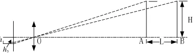
The principle of calibrating the linear CCD’s effective focal length is shown as Figure 1.

2 h 1 h

Figure 1: Principle of calibrating effective focal length

As Figure 1 show, at a position A which is a certain distance away from the camera, sampling

from the calibration template which is

perpendicular to the optical axis. Can readout two

stripes as template which spacing is H occupied

1

h pixels. The relationship can be obtained, such as

(2) from imaging geometry.

H OA dx h

f ₌

1

(2)

In the relationship, OA is the distance between the sampling point A to the camera’s optical center. Because the uncertainty of the camera’s optical center position this distance cannot be accurately measured. Therefore, sample second time by moving template to point B where distance point A

L . Can readout two stripes as template which

spacing is H occupied h₂ pixels from the second

sample picture. The relationship can be obtained, such as (3) from imaging geometry.

H OB dx h

f =

2

(3)

In the relationship, OBis the distance between

the sampling points B to the camera’s optical

center, OB =OA +L. So, the expression of effective

focal length can be obtained by minus (2) to (3) as (4).

H h h

L h h dx f ax

)

( 1 2

2 1 − =

= (4)

3. ANALYSIS OF INFLUENCE FACTORS

3.1 Influence Factors of Optical Center Calibration

The calibration accuracy of optical centers can be

shown as dµ₀ and the corresponding angular

resolution can be demonstrated asd . According to θ

the optical imaging theory applicable to linear CCD, their relationship is supposed to be as (5) shows:

x

a

d

d

/

tan

θ

=

µ

Based on the upright and inverted mirror state theory, the angle measuring accuracy of biaxial tilting table and the resolution accuracy of pixels adopted are the only factors that are related to the angular resolution of the optical center calibration accuracy which equals the sum value of their corresponding angular resolution. The former, related to the digits of the angular coding disk, can

be shown as dϕ and the latter, related to

interpolation precision of the pixels, can be shown

asdγ. Then, calibration accuracy of optical centers

in CCD can be demonstrated in (6):

) tan(

0

ϕ

γ

µ

d = x⋅ + (6)

3.2 Influence Factors of Effective Focal Length Calibration

749

real object height H , the move distance of

calibration model L and the number of image h .

The effect of these factors to the effective focal length calibration result could use their partial differential to represent, as (7) shows.

2 2 1 1

dh h a dh h a dL L a dH H a

da x x x x

x

∂ ∂ + ∂ ∂ + ∂ ∂ + ∂ ∂

= (7)

3.2.1 Impact of real object height

H

The effect of the real object height to the effective focal length calibration could use its differential to represent, after a collation, the result as the (8) shows.

dH H a dH H h h

L h h dH H

ax = x

− = ∂ ∂

2 2 1

2 1

)

( (8)

So, the effects of the real object height H to the

effective focal length calibration will decreases

when H increases. However with the H increases,

the measuring error dH will increase, and in the

real calibration, because of the linear field of view angle of the linear CCD and the calibration

condition, cannot increase the H unlimited. So in

the certain Hcondition, decrease the measuring dH

is the effective way to decrease the effect to the calibration accuracy.

Focus on the calibration of the inner parameter of the linear CCD, all the existing calibration methods are based on the 2D plane, use the black and white streak model to calibrate. This model cannot measure the angle between the linear field of view of the linear CCD and the streak when they are not in the vertical plane. If use the distance of the streak

to approximate estimates the real object heightH,

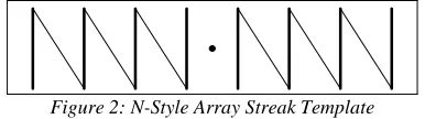
will cause big error for the calculation of the height, and cause large error for the calibration accuracy of the effective focal length calibration. For the measuring the accurate real sampling distance in the calibration model of the linear CCD linear field of view, could use the N-style array streak model to calibrate, as Figure 2 shows.

Figure 2: N-Style Array Streak Template

The point in the center of the Figure 2 locates in the center of the two parallel streaks. It is the sign point in the optical center of the calibration which uses the upright inverted mirror state principle. For distinguish the upright streak and the inclined streak in the image of the linear CCD, the upright streak use the wide line to print. If the linear field

of view of the camera are not in the vertical plane with the upright streak, can use the proportion relationship of the distance between the wide streak and thickness streak in the sampling image, to make sure the real position of the sign point in the inclined streak. Then connect the real position of these sampling points in each inclined streak, this can determine the linear field of view of the linear

CCD real position, and get the accurate distance H

in the calibration model.

Furthermore, according to Figure 1, in the process of the calibration of the effective focal

lengtha , whether the calibration model and the _x

light axe of CCD camera keep vertical will affect

the accuracy for the real object height

measurement. If use the length of the calibration model is 1m, the effect to the real measuring error

dH as the Figure 3 shows.

Figure 3: Effect To The Real Measuring Error dH

750 3.2.2 Impact of number of imaging pixels

h

The calibration impact of the number of imaging pixels of the template in the image h , on the effective focal length can be explained by a differential. The integrated differential is presented in (9) and (10).

1 2 2 1 2 2

1 ( )

dh H h h h dL h ax − = ∂ ∂ (9) 2 2 2 1 2 1

2 ( )

dh H h h h dL h ax − = ∂ ∂ (10)

In (9) and (10), the number of imaging pixels of the template in the image,

1

h and h2, which cannot be changed, is determined by the work distance of sampling image, the actual height of the object, the camera’s focal length, and other parameters. In order to diminish the calibration impact of the number of imaging pixels of the template in the image, h, interpolation of the sub-pixel is utilized, to improve the precision of reading the number of

imaging pixels[11,12]. Matlab has several

interpolation algorithms, including nearest, linear, spline, and cubic, etc. Nearest and linear cannot achieve interpolation of the sub-pixel when calculating the image center. Spline is the most suitable interpolation with the sub-pixel for the 1D interpolation on one row because of its precise.

3.2.3 Impact of translational distance

L

The calibration impact of the translational

distance L of template relative to the linearity CCD

camera can be represented by a differential. The integrated differential is presented in (11).

dL L a dL H h h h h dL L

a_{x x}

= − = ∂ ∂ )

( _{1 2}

2

1 ₍₁₁₎

Hence the longer translational distance L ,the

smaller calibration impact on the effective focal length. However, with the increase of the

translational distance L , its measurement error dL

will be amplified, and during the actual calibration,

the translation distance L cannot be lengthened

infinitely, due to the linear CCD’s depth of field, the conditions of calibration test, and other objective causes. As a result, with fixed

translational distance L , to decrease the

measurement error dLcan effectively neutralize its

impact on the precision of calibration.

From Figure 1, the measurement error dL mainly

comes from the fact if the template translates along the optical axis on the screw rod. In this sense, before conducting a calibration test on the effective focal length, it should be ensured that the mark

point always goes through the optical axis of the linear CCD when calibration template moves on the screw rod, and the template must be maintained vertical to the camera’s optical axis.

4. EXPERIMENTAL DATA

4.1 Accuracy of Optical Center Calibration The focus of a the common linear CCD is 50mm and when we use biaxial tilting tables different in coding digits as well as pixels different in interpolation precision, its calibration accuracy of optical center can be shown in Table 1:

Table.1:The Calibration Accuracy of Optical Center

µ

17 coding digits

18 coding digits

20 coding digits 10-times

interpolation 0.34 0.22 0.13

20-times

interpolation 0.29 0.17 0.08

100-times

interpolation 0.25 0.13 0.04

In the practical process of calibration, we can choose appropriate biaxial tables and pixels according to what we need in reference of data stated in the Table 1.

We choose a 17-digit angular coding disk and 20 times of pixel interpolation accuracy to experiment with the linear CCD whose focus is 50mm and

pixel is 10-2mm. Then we carry out the experiment

according to the upright-down theory, adjusting the focus for a clear image. By adjusting the position of biaxial table and the leading screw, we find that in

the distance from 1m to 3m, the position of

µ

what has been shown in Table 2:

Table.2: Calibration of Optical Center µ₀

distance 1m 1.5m 2m 2.5m 3m

Optical

Center 2047.10 2047.15 2047.15 2047.20 2047.25

It can be know from Table 2 that the calibration error in the experiment is 0.15 pixels and this result concords to what has been figured out in Table 1. It shows a high experimental accuracy.

4.2 Accuracy of Effective Focal Length Calibration

4.2.1 Impact of real object height H

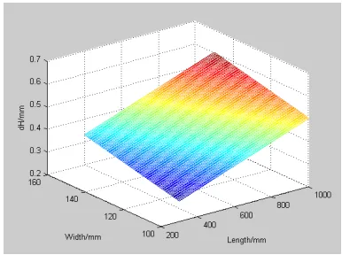
According to (8) and Figure 2 show the principle, can get the fitting graphics of effect in different model size and different streak to the real

measuring error dH through the simulation with the

751

Figure 4: dHOf Black And White Streak Template

As the Figure 4 and Figure 5 show, the real

object height measuring error dH get decrease

when the aspect ratio of the model increase for the black and white streak calibration model, the minimum error is 5mm; the real object height

measuring error dH get increase when the aspect

ratio of the model increase for the N-style array streak calibration model, the maximum error is 0.6mm, the minimum is 0.25mm. So use the N-style array streak model can decrease the measuring error of the real object height, and the effect to the

result of calibration the effective focal length a_x.

Figure 5: dHOf N-Style Array Streak Template

4.2.2 Impact of number of imaging pixels h

Based on (9) and (10), if the work distance of calibration is 1.5m, the translational distance of target surface is 600mm, the template’s height is 1m, and the interpolation algorithm within the sub-pixel is spline, the impact of different sub-pixel’s interpolation precision on the calibration precision of the linearity CCD camera’s effective focal length is elaborated in Figure 6.

Figure 6: Curve Of Impact Of Interpolation Precision

From Figure 6, if the interpolation precision within the pixel is greater than 30 times, a higher interpolation multiple has a small effect on improving the calibration precision of the effective focal length. Besides, the impact on the calibration precision of the effective focal length is very tiny when the error is 0.125 pixels, which is not the major influencing factor. Consequently, based on the requirements of engineering design, choosing interpolation with a 30-time precision within sub-pixel can fulfill the precision requirement of the effective focal length calibration.

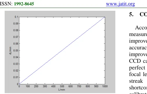
4.2.3 Impact of translational distance

L

The translational distance measurement error curve between the template and linear array CCD camera are as follows. Figure 7 is the curve when

the non-perpendicularity between calibration

template translation and linear array CCD camera

optical axis is1°. Figure 8 is the curve that we using

the method as set in section 3.2.3 which keeps linear array CCD camera optical axis and calibration template perpendicular.

752

Figure 8: dL When Perpendicular

From Figure7 and Figure 8, the measurement

error of translation distance L is proportional to

itself. The translational distance L has a higher

measuring accuracy under condition that the calibration template and line array CCD camera optical axis are perpendicular.

4.2.4 Experiment of effective focal length calibration

Based on the analysis of actual height H ,

number of pixels h and translational distance L,

we calibrate with a length of 300mm, width 200mm N-style array streak calibration template at about 1m distance from linear CCD, and sample once in each translation 300mm. Then get the actual height of the object. H=324.3mm. Use 30 times sub-pixel interpolation precision to obtain the number of

imaging pixel h in each sampling location, as

shown in Table 3.

Table 3: The Number of Imaging Pixel h

Translational

distance 0mm 300mm 600mm 900mm

h 1614.70 1247.93 1017.40 858.67

Based on the effective focal length calculation principle shown in (4), we can obtain the effective

focal length a_x calibration results shown in Table 4.

Table 4 : The Effective Focal Length a_x Calibration Results

loca tion

0/ 300

0/ 600

0/ 900

300/ 600

300/ 900

600/ 900

x

a 5082 .3

5088 .6

5089 .5

5094. 8

5093 .1

5091 .4

From the results of Table 4, the experimental results of calibration error are 0.13 pixel units. Calibration accuracy is about 2.5‰. This is an effective way to improve the accuracy of the effective focal length of the linear CCD calibration.

5. CONCLUSION

According to the theory of error analysis and measurement results, in this article, the analysis and improvement of the internal parameters calibration accuracy factor of linear CCD’s calibration has improved calibration accuracy of the linear array CCD camera internal parameters at lower cost and perfect experimental. Especially in the effective focal length of the calibration, using N-style array streak calibration template has overcame the shortcomings of the cycle of black and white streak calibration template which could not accurately determine the linear array CCD camera liner field of view position. This improved the measurement accuracy of the actual height. Deficiency in this article was that the linear CCD lens distortion has not been taken into account. So calibration experiments could not reach the theoretical precision values. The accurate calibration of the effective focal length parameters would be more accurate if the lens distortion parameters had been used to correct the position of the imaging in effective focal length calibration.

REFERENCES:

[1] Zhiyong Lei, Shoushan Jiang, “Liner scan CCD

technology and its application in target measurement”, Journal of Xi’an Institute of

Technological, Vol.22, No.3, 2002, pp.220-224.

[2] R.Y. Tsai, “A versatile camera calibration

technique for high-accuracy 3D machine vision metrology using off-the-shelf TV cameras and lenses”, IEEE Journal of Robotics and

Automation, Vol.3 No.4, 1987, pp323-344.

[3] Z. Zhang, “A flexible new technique for camera

calibration”, Technical Report MSR-TR-98-71, Dec.2, 1998.

[4] Hong’e Luo, Ping Chen, “A new method of lens

distortion calibration of linear CCD

measurement system”, Semiconductor

Optoelectoronics, Vol.30, No.3, 2009,

pp.441-443.

[5] C.A. Luna, M. Mazo, “Calibration of line-scan

cameras”, IEEE Transactions on

Instrumentation and Measurement, Vol.59,

No.8, 2010, pp.2185-2190.

[6] Xiang Chen, Kun Wei, “Automatic calibration

in sual linear-CCD camera intersection

measuring system”, Science of Surveying and

753

[7] L.D. Light, “The new camera calibration system

at the U.S. Geological Survey”,

Photogrammetric Engineering & Remote

Sensing, Vol.58, No.2, 1992, pp.185-188.

[8] X. Cao, H. Foroosh, “Camera calibration using

symmetric objects”, IEEE Trans. On Image

Processing, Vol.15, No.11, 2006,

pp.3614-3619.

[9] Dong Wang, Ming Zhu, “Camera’s image

center measurement method based of gistorted symmetry”, Chinese Journal of Electron

Devices, Vol.30, No.3, 2007, pp.1003-1005.

[10] Dianguo Cao, Haojie Chen, “Application of

bilinear interpolation algorithm in image rotation based on matlab”, China Printing and

Packaging Study, Vol. 2, No.4, 2010, pp.74-78.

[11] Qingying Wang, “Deduction on the formula of

depth of field”, Journal of Nanyang Teachers’

College (Natural Sciences Edition), Vol.2, No.3,

2003, pp.24-26.

[12] K. Juho, B. Sami, “A genertic camera model

and calibration method for conventional, wide-angle, and fish-eye lenses”, IEEE Trans. On

Pattern Analysis and Machine Intelligence,