2132
ALTERNATING SENSING PROCESS TO PROLONG THE
LIFETIME OF WIRELESS SENSOR NETWORKS
1MOHAMMED AL-SHALABI, 2MOHAMMED ANBAR, 3ALAA OBEIDAT
1,2National Advanced IPv6 Center, Universiti Sains Malaysia, Penang, Malaysia 3Basic Sciences Department, the Hashemite University, Zarqa, Jordan
E-mail: 1[email protected], 2[email protected], 3[email protected]
ABSTRACT
In the last few decades, the usage of Wireless Sensor Networks (WSNs) is dramatically increased due to the nature of this type of networks where the nodes are randomly deployed in a large area to sense some attributes which the human beings cannot do so and send the data to the main device called Base Station (BS), and this process takes a time interval called round. The deployed nodes may be located near to each other and then they may sense approximately the same events. The process of sensing and sending the same data to the BS consumes a lot of energy in the nearby nodes and they will die fast. An alternating sensing process is proposed. The goal of the proposed mechanism is to prolong the lifetime of the network by increasing the lifetime of the nearby nodes and reducing the consumed energy in them. This goal is achieved by scheduling the sensing process to reduce the consumed energy as much as possible. The MATLAB tool is used to evaluate the proposed mechanism and compare it with the LEACH protocol. The results show that the proposed mechanism outperforms the LEACH protocol in terms of the network lifetime and the number of transmitted packets to the BS by approximately 9% and 17% alternatively.
KEYWORDS: Wireless Sensor Networks, Network Lifetime, Sensing Process, Nearby Nodes, Leach
Protocol.
1. INTRODUCTION
Wireless Sensor Networks (WSNs) provides an efficient way for monitoring many applications such as underwater monitoring and fire prediction to reduce the risk on human beings. Sensors move the physical world to digital world by catching the required phenomena in the real-world and send them digitally for further processing to the main device called Base Station (BS) [1].
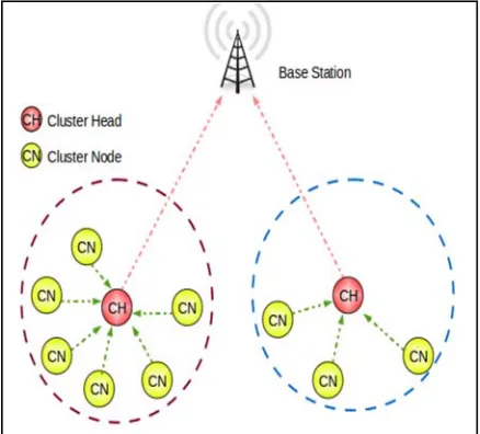
In order to do the WSNs their works efficiently, there are many routing protocols are proposed to handle the way of sending the data from sensor nodes to the BS. There are three classes of routing protocols based on the network’s structure: Flat Routing, Hierarchical-based Routing and Location-based Routing protocol [2]. The most important class is the Hierarchical-based Routing class, where the network is divided into several groups called ‘Clusters’ and each cluster has one basic node called Cluster Head(CH) and many sensor nodes. The task of the CH is to collect the data from other sensor nodes in the cluster, aggregate them and
[image:1.612.316.535.491.689.2]send the aggregated data to the BS [3]. Figure 1 illustrates the structure of this type of routing protocols.
Figure 1: Hierarchal-based routing protocols
2133 one node (CH) and send them at one time. Moreover, these protocols fairly consume the energy in the nodes by distributing the role of the CH among the nodes [4]. Some of the hierarchical protocols that have been proposed for sensor networks are the LEACH protocol [5], Power-Efficient Gathering in Sensor Information Systems (PEGASIS) [6], Threshold-Sensitive Energy-Efficient Sensor Network (TEEN) [7], and Adaptive Threshold-sensitive Energy-Efficient sensor Network (APTEEN) [8], in addition to many variants of LEACH protocol.
Next section discuss the LEACH protocols in details due to its importance in the hierarchical-based routing protocols, and to understand how this protocol works in order to inspire the proposed sensing process from it.
1.1 LEACH Protocol
The LEACH protocol [5] is considered as the main hierarchical-based protocol, and the first energy efficient routing protocol that is proposed to prolong the WSN’s lifetime. LEACH protocol consists of two stages, the first stage is the set-up, and the second stage is the steady-state. In the set-up phase, each node creates a random number between 0 and 1 and compares this value with a threshold value, if this value is less than the threshold value, then this node will be a CH. Threshold value is calculated according to the following formula [9]:
T n if n ∈ G
0 otherwise (1)
Where p is the percentage of CH, r is the current
round, and G is the group of sensor nodes that are
not CHs in the previous 1/p round [9].
Nodes that will be CHs send a message to all sensor nodes in the network, and then each sensor node decides its CH according to the strength of the received message and sends a joint message to the CH. After that, the clusters formed, and the CH creates a Time Division Multiple Access (TDMA)
schedule according to the number of nodes in the cluster, then it sends this schedule to all nodes in the cluster [9].
In the steady-state phase, sensor nodes starts sensing, then each sensor node sends its data to the CH using its time slot, the CH aggregates the received data and sends them to the BS [9]. The unit of time for the set-up and the steady-state phases is called ‘round’, and the same procedure
will be repeated in each round.
The process of sensing data will be done by each sensor node in each cluster every round, and due to the nature of the hierarchical-based routing protocols, the role of the CH is distributed among nodes, and the clusters are formed again every round. As a result of these processes, the locations of the CHs are changed, and if a CH sends large amount of data to the BS, it consumes its energy very fast and this negatively affects the lifetime of a network especially if the data which are sent by nearby nodes are redundant.
The aim of the proposed mechanism is to reduce the amount of energy which is consumed during the sensing process in the nearby nodes by scheduling the sensing process in an efficient way. Reducing the consumed energy leads to increase the lifetime of the nearby nodes and then the whole network. The nearby nodes are selected to be considered because there is a shared area between any two nearby nodes, and the events in this area are sensed by each nearby node, which leads to consume a large amount of energy. The proposed mechanism is described in details in section 3.
Many protocols are suggested to handle the sensing process in order to save the energy in the nearby nodes as much as possible. Next section describes the related protocols.
2. RELATED WORKS
2134 overcome the limitation of LEACH in considering the distance between nodes in the sensing process.
Authors in [10] have proposed a coverage aware protocol for WSNs to schedule the sleeping of nodes based on the shared area with adjacent nodes. The proposed protocol considers increasing the number of sleeping nodes and minimizing the number of active nodes in order to increase the network’s lifetime. The nodes those have equal sensing range start sleeping while keeping one node in active mode. The proposed protocol gives good performance in terms of coverage efficiency but it does not give a clear vision about the sleeping scheduling process.
Sleep Scheduled and Tree-Based Clustering Routing Protocol (SSTBC) is suggested in [11] to maximize the network lifetime by preserving energy in the deployed sensor nodes. Authors of [11] select the nodes to turn off their radio based on a threshold, which is the size of the grid divided to preserve the energy. The sensing area is divided into square grids, and the nodes which have highest residual energy still active while other nodes are in sleep mode in the same grid for the current round.
Random Back off Sleep Protocol (RBSP) is proposed in [12] to schedule the active and sleep modes in WSNs. RBSP is based on the residual energy of the active nodes, and each active node determines its sleeping window based on its residual energy. The size of the sleeping window determines the probability of turning on of the neighbor nodes. Neighbor nodes use the sleeping window information from the active node to determine its sleep time.
Multi Working Sets Alternate Covering (MWSAC) protocol is proposed in [13] in order to reduce the energy consumption in the sensor nodes in WSNs. Authors of this protocol proposed a distributed algorithm in the first stage to create the maximum number of working sets to accomplish the partial coverage requirement. In the next stage, the sleeping schedule is set by making the nodes in the same working set wake up synchronously while the nodes in multiple working sets wake up asynchronously. Therefore, when the nodes in any working set are waking, nodes in other sets are sleeping to save the energy.
To summarize, the abovementioned protocols are proposed to preserve the energy in the sensor nodes by scheduling the sleeping and active modes.
However, there are still gaps in the related protocols such as the dependency on the residual energy of nodes without considering the distance between them. Another gap is the computation overhead when increasing the calculations and processing such as the spanning tree construction which requires more energy. Moreover, the coverage is still not efficiently considered in the related protocols, which is very important when taking about the sleeping and active schedule to make the sensing process of the network as stable as possible and do not loss any event without sensing as much as possible.
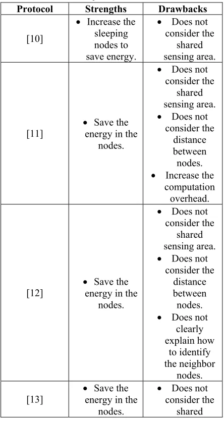
[image:3.612.307.529.321.740.2]The following table illustrates the above mentioned protocols with their strengths and drawbacks.
Table 1: Previous works on sleeping scheduling protocols.
Protocol Strengths Drawbacks
[10]
Increase the sleeping nodes to save energy.
Does not consider the
shared sensing area.
[11] energy in the Save the nodes.
Does not consider the
shared sensing area.
Does not consider the
distance between nodes.
Increase the computation overhead.
[12] energy in the Save the nodes.
Does not consider the
shared sensing area.
Does not consider the
distance between nodes.
Does not clearly explain how
to identify the neighbor
nodes.
[13] energy in the Save the nodes.
Does not consider the
2135 sensing area.
Increase the computation overhead by
adding previous
stage.
The proposed mechanism covers the gaps in the previous studies by considering the shared area (grey area) to schedule the sensing process because this area contains events to be sensed by the nearby nodes. In this case, each node senses the same events in this area and sends the same information to the BS, this leads to consume a lot of energy in these nodes and then die quickly. The proposed mechanism highlights the shared area and utilizes it to prolong the network lifetime.
3. METHODOLOGY
As discussed earlier, the sensing process strongly affects the performance of the network in terms of its lifetime specially if there are many nearby sensor nodes. This negative effect should be reduced as much as possible to prolong the lifetime of a network by saving the energy of the nearby nodes as much as possible. The proposed sensing process in this paper considers this issue and can prolong the lifetime of the network by handling the sensing process in the nearby node.
Before starting with the proposed sensing process, the nearby nodes should be identified mathematically and then apply the proposed sensing process on them. The following subsections discuss these aspects in details.
3.1 Nearby Nodes Identification
In the proposed sensing process, the sensor nodes are randomly distributed in a region, and the nearby nodes are identified by the BS based on the distance between them in the whole network. The distance between nodes based on the radius of them, with the note that the radius is the same for all nodes because they are homogeneous. After identifying the nearby nodes, they are divided into two groups, A and B, to handle the alternating sensing process by assigning a slot of time for each group as will be described in the next subsection.
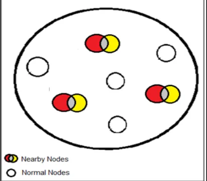
Figure 2 represents the nearby nodes in a cluster based on the distance between them.
Figure 2: Nearby nodes
In figure 2, the nearby nodes which are colored with red and yellow, are identified by the BS as described in the following paragraphs.
All nodes have the same radius R since they
are homogeneous. The BS takes the decision of grouping based on the predefined threshold. If the distances between nodes satisfy this threshold, the BS starts grouping them into two groups, A and B. The BS knows the coordinates of each node in the network and stores this information with other
information such as the energy of each node in the array data structure.
In the proposed process, and to avoid the extra messages’ overheads and calculations, the nodes do not have any information about the locations of their neighbors. Furthermore, using mechanisms to find the locations of nodes such as GPS is energy consumed, for these reasons; just the BS can find the locations of nodes and identify them. In fact, what concerns the proposed process is not how the BS knows the locations of the nodes, there are many techniques to specify the locations, but the proposed process starts after the BS stores the basic information initially in the array data structure.
After getting the coordinates of the nodes by the BS, it starts finding the distance between them and identifies the nearby nodes. The BS uses a predefined threshold value Td to determine if any
two nodes are nearby nodes or not as explained in (2).
[image:4.612.313.519.271.451.2]2136 Where Td is the threshold value and r is the radius
of the sensing area.
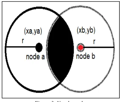
Identifying node a and node bas nearby nodes
is based on the value of Td, If the distance from
node a to node b is less than or equal the threshold
value Td, which is calculated using (2), then the
[image:5.612.102.299.209.376.2]two nodes are nearby as shown in figure 3.
Figure 3: Nearby nodes
The following equation describes this situation:
D a, b 𝑇𝑑 (3)
Where D(a,b) is the Euclidean distance between
node a and node b and is given in (4).
D xa, ya , xb, yb xa xb ya yb
(4) where(xa, ya)and (xb,yb) are the coordinates of
nodes a and b respectively.
If the distance from one node to another node is more than the threshold Td, then the two nodes
are not nearby, and if the distance between them is less than Td, then the two nodes are nearby.
Equation (5) shows the probability of two nodes to be nearby.
O 1 if D a, b Td
0 if D a, b 𝑇𝑑 (5)
Where O is the Boolean variable that indicates
whether nodes a and b are nearby, D(a,b) is the
distance from node a to node b as explained in (4),
and Td is the distance threshold as explained in (2).
In the following subsection, the proposed sensing process is discussed in details.
3.2 The Proposed Sensing Process
In the case of nearby nodes, there is a shared area between them, and if they start the sensing process together, then they sense the same events which occur in the shared area at the same time and transmit the same sensed data to the BS, this will waste energy and makes the nearby nodes die quickly. In addition, data redundancy will occur in the BS, so there is no need for both nearby nodes to sense the same events at the same time. Hence, in the proposed process, and to solve this problem, the nearby nodes in the clusters start the sensing process in an alternating manner by assigning a slot of time for each nearby node.
After ending of identifying and grouping the nearby nodes, the sensing process will start. For example, node i (group A) senses the events on its
sensing area and node j (group B) is in sleep mode,
after ending the sensing time of time i, it will send
the sensed data to its CH and node j doesn’t send
anything. Then, node i will be in sleep mode, and
node j starts its sensing time for sensing the events
in its sensing area. Afterwards, node j sends the
sensed data to its CH. In this way, the energy consumption in the nearby nodes reduces, and also reduce the redundancy of data that are sent to the CHs, because if node i and node j sense the same
event which is located in the shared sensing area at the same time, then the collected data of that event are the same and the two nodes send approximately the same data or at least send a high percentage of redundant data to the BS. This process is done for all nodes in each group.
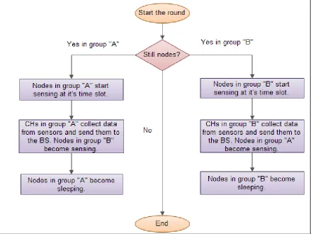
2137 At a specific point, the sensor nodes in group “A” stop sensing of data and start sending them to the CHs, then the CHs begin sending the gathered data to the BS. During that, the sensor nodes in group “A” start the sleep mode. At the same time, the sensor nodes in group “B” begin the active
[image:6.612.91.530.280.610.2]mode and start sensing the data. Figure 4 shows the flowchart of the alternating sensing between the groups.
Figure 4: Organize the sensing process between Groups
From Figure 4, it is shown that when the CHs in group “A” start sending data to the BS, sensor nodes in group “A” become in sleeping mode, while nodes in group “B” become in active mode and start sensing, and vice versa. The alternating of the sensing process between the groups helps to
maintain the energy in the nearby nodes, which leads to increase the lifetime of these nodes, and as a result, it leads to prolong the lifetime of the whole network.
4 SIMULATION RESULTS AND COMPARISON
In the proposed mechanism, the lifetime of the whole network is very important metric to evaluate the performance of it. The nearby nodes in the network are considered critical nodes due to their
importance in the proposed mechanism. Therefore, the lifetime of these nodes determines the lifetime of the whole network.
The lifetime of the network is measured using different methods [14]. The method which is used
2138 the CHs, because this value indicates that there are active nodes sending data to the BS for long time. Moreover, the reliability and the efficiency of the network increase.
The metrics used in this paper to evaluate the proposed mechanism and compare it with the LEACH protocol are listed in table 2.
TABLE 2:EVALUATION METRICS
Metric Description LND Last Node Die (rounds) Packets to BS Number of packets sent to the BS by the CHs.
The comparison is done with the LEACH protocol because it is considered as the main clustering protocol, and the proposed mechanism enhances it. Moreover, the related methods which enhance the LEACH protocol did not consider the nearby nodes, even the methods which consider the sensing process. For these reasons, the comparison with these methods is not fair and dos not evaluate the proposed mechanism in an accurate manner.
Table 3 presents the main considered parameters for simulating the proposed mechanism. These parameters based on the previous studies and the LEACH protocol.
Table 3: Simulation Parameters
Symbol Description Value
A Network size 100 X 100
BS (i,j) Position of the base station (50,50)
N Number of nodes 100
Eo Initial energy 0.5 Joule
Eamp Transmit amplifier pJ/bit/m2 13
Eelec Electronic energy consumption 50 nJ/bit
Erx Reception energy 50 nJ/bit Etx Transmission energy 50 nJ/bit Eda Data aggregation energy 5nJ/bit
Rmax Maximum number of rounds 10000
R Radius of each node 1 m
The simulation is done using the MATLAB as a simulator tool, and it is done for 30 times to get accurate results and to reduce the effect of the randomness in the nodes’ distribution. Moreover, the proposed mechanism and the LEACH protocol are applied on the same network topology and the same positions of nodes in each run to get fair results.
When starting each run, the nodes are randomly distributed on the area A and the nearby
nodes are identified as shown in figure 5.
Figure 5 shows the nearby nodes in red and yellow colors, and these nodes join groups A and B.
After that, the alternating sensing process starts. This procedure is repeated in each round. The results of the simulations based on the metrics in table 2 are presented in the following figures.
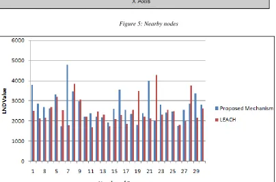
Figure 6 shows the LND values for the proposed mechanism and the LEACH protocol in 30 runs.
2139
[image:8.612.91.523.58.569.2]
Figure 5: Nearby nodes
Figure 6: Comparison based on LND metric
Based on figure 6, the average of the LND values in the proposed mechanism is 2706, while in the LEACH protocol is 2488. These values indicate that the lifetime is increased by 219 rounds, which is approximately 9%, in the proposed mechanism. This increment in the lifetime is due to the efficient
alternating sensing process that saves the energy in the nearby nodes.
[image:8.612.99.503.323.589.2]2140
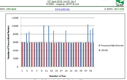
Figure 7: Comparison based on Packets to BS metric
Figure 7 shows that the average number of the transmitted packets from the CHs to the BS in the proposed mechanism is 6933 packets, and in the LEACH protocol is 5904 packets, with increment of 1029 packets in the proposed mechanism (approximately 17%). The increasing number of the transmitted packets in the proposed mechanism indicated that the alive nodes are still active and sending data to the BS for long time, which increases the efficiency of the network.
5 CONCLUSIONS
In a WSN, the process of sensing significantly impacts its performance. Several studies have been conducted to deal with this problem. In this paper, an alternating sensing process is presented to reduce the consumed energy and prolong the WSN’s lifetime by considering the shared area between nearby nodes and schedule the sensing process between them. The proposed mechanism outperforms the LEACH protocol in terms of the network lifetime and the number of transmitted packets to the BS. Based on the simulation values, the proposed mechanism increases the lifetime of the network and the number of the transmitted packets to the BS by approximately 9% and 17% alternatively. The future work will consider the implementation of the proposed process using the MATLAB simulation tool, in addition to the evaluation of it compared with the related works.
The proposed mechanism considered the static nodes in the WSNs. In the future, the mobile nodes will be considered to prolong the lifetime of the MANET (Mobile Ad Hoc Networks).
REFERENCES
[1] D. Culler, D. Estrin, M. Srivastava, "Overview of Sensor Networks", IEEE Computer USA, vol.
37, pp. 41-49, August 2004.
[2] Ameer Ahmed Abbasi a, Mohamed Younis, "A survey on clustering algorithms for wireless sensor networks", Computer Communications,
vol. 30, pp. 2826-2841, 2007.
[3] J. J. Lotf, M. Hosseinzadeh, and R. M. Alguliev, “Hierarchical routing in wireless sensor networks: a survey,” in Computer Engineering and Technology (ICCET), 2010 2nd International Conference on, vol. 3, April 2010, pp. V3–650–V3–654.
[4]V. K. Arora, V. Sharma, and M. Sachdeva, “A survey on LEACH and others routing protocols in a wireless sensor network,” Optik - International Journal for Light and Electron Optics, vol. 127, no. 16, pp. 6590–6600, 2016.
2141 [6] S. Lindsey and C. Raghavendra, “Pegasis:
Power-efficient gathering in sensor information systems,” in Aerospace Conference Proceedings, 2002. IEEE, vol. 3, 2002, pp. 3– 1125–3–1130 vol.3.
[7]A. Manjeshwar and D. P. Agrawal, “Teen: a routing protocol for enhanced efficiency in wireless sensor networks,” in Parallel and Distributed Processing Symposium., Proceedings 15th International, April 2001, pp. 2009–2015.
[8] Manjeshwar, A., &Agrawal, D. P. (2002). APTEEN: A hybrid protocol for efficient routing and comprehensive information retrieval in wireless. In Proceedings - International Parallel and Distributed Processing Symposium, IPDPS 2002 (p. 195).
[9]Heinzelman W. B., Chandrakasan A. P., Balakrishnan H., ”An application-specific protocol architecture for wireless microsensor networks,” IEEE Trans on Wireless Communications, Vol. 1, No.4,2002, pp. 660-670, doi: 10.1109/TWC.2002.804190.
[10] U. Pacharancey, A. Shaikh, P. Jadhav, and M. Madankar, “Coverage Aware Sleep Scheduling in Wireless Sensor Networks”, Int. J. Sc. Res. In Network Security and Communication (IJSRNSC), Vol. 5, pp. 20-23, May 2017.
[11] Tan, N.D. and Viet, N.D., 2015, January. SSTBC: Sleep scheduled and tree-based clustering routing protocol for energy-efficient in wireless sensor networks. In Computing & Communication Technologies-Research, Innovation, and Vision for the Future (RIVF), 2015 IEEE RIVF International Conference on (pp. 180-185). IEEE.
[12] More, A. and Raisinghani, V., 2014. Random backoff sleep protocol for energy efficient coverage in wireless sensor networks. In Advanced Computing, Networking and Informatics-Volume 2 (pp. 123-131). Springer, Cham.
[13] Huang, M., Liu, A., Zhao, M. and Wang, T. (2018). Multi working sets alternate covering scheme for continuous partial coverage in WSNs. Peer-to-Peer Networking and Applications.