R E S E A R C H
Open Access
Cardiology knowledge free ECG feature
extraction using generalized tensor rank one
discriminant analysis
Kai Huang
*and Liqing Zhang
Abstract
Applications based on electrocardiogram (ECG) signal feature extraction and classification are of major importance to the autodiagnosis of heart diseases. Most studies on ECG classification methods have targeted only 1- or 2-lead ECG signals. This limitation results from the unavailability of real clinical 12-lead ECG data, which would help train the classification models. In this study, we propose a new tensor-based scheme, which is motivated by the lack of effective feature extraction methods for direct tensor data input. In this scheme, an ECG signal is represented by third-order tensors in the spatial-spectral-temporal domain after using short-time Fourier transform on the raw ECG data. To overcome the limitations of tensor rank one discriminant analysis (TR1DA) inherited from linear discriminant analysis, we introduced a generalized tensor rank one discriminant analysis (GTR1DA). This approach involves considering the distribution of the data points near the classification boundary to calculate better projection tensors. The experimental results showed that the proposed method achieves greater classification accuracy than other vector- and tensor-based methods. Finally, GTR1DA features a better convergence property than the original TR1DA.
Keywords: ECG analysis; Feature extraction; Tensor learning approaches; Dimension reduction; TR1DA
1 Introduction
As the Internet of Things technology matures, remote and centralized electrocardiogram (ECG) diagnostic forms have been developed. A highly centralized plat-form has a large amount of ECG data to diagnose daily; therefore, an aided diagnosis system providing reference diagnostics is beneficial. An ECG represents the work-ing state of the heart by recordwork-ing the magnitude and direction of the electrical activities related to the heart. It provides useful information for doctors to diagnose heart diseases. In recent years, the automatic diagnosis of heart diseases through the analysis of ECG signals has drawn much attention. ECG feature extraction consists of deter-mining a set of discriminant features to represent ECG data to achieve strong classification performance. Many technologies and algorithms on machine learning and sig-nal processing have been used to achieve this goal. Zhao
*Correspondence: [email protected]
The MOE-Microsoft Key Laboratory for Intelligent Computing and Intelligent Systems, Department of Computer Science and Engineering, Shanghai Jiao Tong University, Shanghai 200240, China
et al. proposed a feature extraction method using wavelet transform [1]. Jen et al. described an approach that takes advantage of the neural networks for determining the fea-tures of a given ECG signal [2]. Pasolli et al. introduced an active learning method for ECG classification based on certain ECG morphology and temporal features [3]. Zhang et al. used the principal component analysis (PCA) algorithm to extract ECG features [4]. An ECG feature extraction scheme using independent component analysis (ICA) was presented by Wu et al. [5,6].
The main problem with the existing methods is their limitation to 1- or 2-lead ECGs because a public 12-lead ECG database is lacking. Traditional methods developed for 2-lead signals cannot be directly applied to 12-lead ECG signals. They typically use vectors to represent ECG signals; however, this is not a natural representation of ECG signals because a large amount of useful structural information is discarded. The structural information indi-cates the relative positions of the signals among differ-ent leads. The 12-lead ECG provides spatial information about the electrical activity of the heart in three approxi-mately orthogonal directions. If all the information of the
12-lead signals is considered, then robust features can be obtained and then used for an automatic analysis. Thus, a high classification accuracy and an efficient representa-tion of the ECG signals can be achieved. Moreover, the time-frequency domain features can also help improve the effect of the classification. Therefore, our method involves converting an original 12-lead ECG signal into a spatial-spectral-temporal domain such that it becomes a third-order tensor.
Scanning all tensor ECG signals into a vector greatly increases the dimensions of the feature space. Conse-quently, the number of training samples seems extremely small compared with the large dimensions of the feature space; this problem is called the small sample size (SSS) problem [7]. Another problem is related to the number of unknown parameters that can lead to an overfitting prob-lem according to the principle of Ockham’s razor. There-fore, the objective is to use the tensor feature extraction method to retain as much of the data structure informa-tion as possible. A more natural method to represent ECG compared with vectorization is to use third-order tensors. If the appropriate technology is adopted, then additional information can be extracted from the ECG data, and, therefore, the SSS problem can be addressed. Li et al. suc-cessfully used a general tensor discriminant analysis for single-trial electroencephalogram (EEG) classification [8]. This approach has also been adopted in gait recognition [9]. Other tensor methods include multilinear principal component analysis (MPCA) [10,11], uncorrelated multi-linear PCA (UMPCA) [12,13], and tensor rank one dis-criminative analysis (TR1DA) [14]. These approaches can be classified into two categories [15]: the methods corre-sponding to tensor-to-tensor projection and the methods corresponding to tensor-to-vector projection. GTDA [9] and MPCA [10,11] belong to the tensor-to-tensor cate-gory, whereas TR1DA [14] and UMPCA [12,13] belong to the tensor-to-vector projection category. Because TR1DA is an extension of linear discriminant analysis (LDA), it also exhibits the same limitations. More precisely, it does not enable the characteristics of the original data distri-bution and adjacent points of the different classes to be fully considered. In this study, we propose to improve the original TR1DA method and overcome its limitations. We therefore consider the distribution of the closing points of the different classes to calculate better projection tensors and improve the accuracy of the classification.
In this paper, we introduce a new tensor-based scheme to extract features from 12-lead ECG signals. We repre-sent them using high-order tensors, i.e., 12-lead signals in the spatial-spectral-temporal domain. The tensors were constructed using short-time Fourier transform (STFT) on the raw ECG signals. Generalized TR1DA (GTR1DA) was used to reserve the projection tensors from which the features of the original tensors were obtained. Finally,
a support vector machine (SVM) with Gaussian kernel was used for the classification in the feature space. We tested the proposed method on our patient database and achieved a high classification accuracy.
The paper is organized as follows. The data preprocess-ing approach and the tensor data achievement process are introduced in Sections 2.1 and 2.2, respectively. We then discuss the tensor calculation used in this paper in Section 3. Section 4 indicates the major limitations of LDA, and Section 5 introduces an extension of LDA. In Section 6, the main idea of TR1DA is presented. We then show how to generalize the original TR1DA into GTR1DA in Section 7. Section 8 justifies the proposed method. In Section 9, we introduce the initial value calcu-lation used in our approach. In Section 10, we clarify and briefly explain how SVM was applied for multiclass clas-sification. We then briefly introduce our ECG database in Section 11.1 and describe the convergence improve-ment and the accuracy of the classification in Section 11.2. Section 12 presents the conclusion.
2 Tensor-based scheme
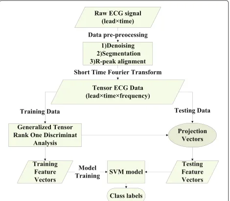
Our work covered the data preprocessing, the tensor data computation using STFT, the tensor feature extraction and dimension reduction based on our new GTR1DA approach, and the classification of the multiclass. The block diagram is provided in Figure 1.
2.1 Data preprocessing
Raw ECG signals typically display strong background noise. To suppress the noise without ruining the data, we used common methods, such as wavelet transforma-tion, to remove high-frequency noise and median filters
to eliminate the baseline drift. An ECG signal from a diag-nosis is approximately 20 s long and comprises approxi-mately 25 beats. Therefore another critical preprocessing step is to segment the signal into ‘ECG pieces’, each of which contains one heartbeat.
2.2 Short-time Fourier transform
The original signals represent the features in the spatial-temporal domain. Because ECG signals are nonstation-ary, we used STFT [16] instead of the regular Fourier transform to collect information on when a particular frequency component occurs. STFT can provide useful information regarding the time resolution of the spec-trum. STFT involves extracting several frames from the signals and analyzing them using a time-sliding window such that the relation between the variation of the fre-quency and the time can be identified. We used STFT to transform the original signals into a spatial-spectral-temporal domain as high-dimensional third-order tensors [17]. Given a signal that varies over time, STFT was used to determine the sinusoidal frequency and phase the content of the local sections.
For a 12-lead (lead× time) ECG signal sample,s[l,n] represents the discrete-time signal at a timenfor a leadl. Then, the STFT at a timentand a frequencyfis given by
STFT{s[l,n]}(m,w)≡S(l,m,n)
=m∞=−∞ω(n−m)s(l,m)e−j2πfm (1)
wherew[n] is the window function that selectively deter-mines the portion ofs[l,n] to use for the analysis. In this study, we used the Hann window. Once STFT had been applied to the ECG signals, all of the signals were in a third-order tensor form for the remainder of the analy-sis. In accordance with previous studies on extending an EEG signal to a third-order tensor [18-20], we extended the original ECG signal such that we could effectively extract valuable features in the spatial-spectral-temporal domain. To appropriately manage this type of data, using a tensor-based learning approach was necessary.
3 Tensor operations
We first introduce definitions of tensor operations to fix the notations. In our paper, Mathcal font and upper-case letters denote tensors (e.g., X,Y,Z). Matrices are expressed as bold uppercase letters (e.g.,X,B). Lowercase bold letters are used for vectors (e.g.,u,a). Lowercase and uppercase letters are scalers (e.g.,a,b,c,D,E).
Definition 1.Tensor product. The tensor product of two vectorsx∈RMandy∈RNis a matrix:
(x⊗y)ij=xi×yj, (2)
which is a rank 1 tensor of mode 2. Here, 0 < i ≤ M and 0 < j ≤N. The tensor product of three vectorsx ∈ RMy∈RN, andz∈RSis a mode-3 tensor:
(x⊗y⊗z)ijk =xi×yj×zk, (3)
which is also of rank 1. Here, 0<i≤M, 0<j≤N, and 0<k≤S.
Definition 2.Tensor mode product. A modeMtensor
X of sizeX ∈ RN1×N2×...×NM multiplied by a vector in
moderis a tensor with a size ofN1×N2×. . .×Nr−1× 1×Nr+1×. . .×NM:
(X×ru)i1×i2×...×ir−1×1×ir+1×...×iM
=
ir
(Xi1×i2×...×ir−1×ir×ir+1×...×iMuir), (4)
which is a tensor of modeM−1.
Definition 3.Multiple tensor product. The tensor prod-uct of multiple vectors forms a rank 1 tensor. To simplify its notation, we use the following form to represent the tensor product of several vectors:
u1⊗u2⊗. . .⊗un= M
l=1
⊗(ul)T. (5)
4 Limitations of classical linear discriminant analysis
In this section, we review the main limitations of classi-cal LDA, including the SSS problem, the low-rank prob-lem, the heteroscedastic probprob-lem, the problem raised by the unreasonable between-class scatter matrix, and the unconsidered distribution structure between classes.
4.1 Small-size problem
In the classical LDA approach, the calculation of the ratio of the between-class covariance distance to the within-class covariance distance is a generalized Rayleigh quo-tient problem. We illustrate it using the most widely used optimization problem, which is the first optimization problem in Equation 6.
R(x)= x
TS bx
xTSwx,R(x)= xTSbx
xTStx,R(x)= xTSwx
xTStx. (6)
The Lagrange multiplier method can be used to solve this problem. It is clear from Equation 6 that xhas an infinite number of solutions. Whenxis multiplied by a constant,R(x)maintains the same value (only offsetting the numerator and denominator). Therefore, the length of
restriction is used as a condition for the Lagrange method. The solution to this problem maximizes the equation:
c(x)=xTSbx−λ(xTSwx−1)
⇒ dc
dx=2Sbx−2λSwx=0 ⇒Sbx=λSwx.
(7)
The above equation is a typical generalized eigenvalue problem. If the within-class scatter matrixSwis invertible,
this problem can be converted into an ordinary eigenvalue problem, allowing us to calculate the result:
Sw−1Sbx=λx (8)
The within-class scatter matrix is the sum of each class covariance matrix, and rank(C) ≤ rank(A) +rank(B); therefore, the rank of the within-class scatter matrix is at most s (the number of classes) less than the sample number.
In most cases, such as image processing, video analy-sis, FMRI, or CT, the dimensions of the original signal are considerably large. However, if the training set is exces-sively small and the number of cases is less than the dimension count, the application of LDA is limited, and modifications are required to solve the problem.
4.2 Class number 1: low-rank problem
The classical LDA approach involves calculating the between-class scatter matrix by computing the covariance matrix of each class data center.Hbcan also be expressed
in the following form:
Hb=
1
√
n
C(1),C(2),. . .,C(i),. . .,C(s)
C(i)=
(c(1i)−c),(c(2i)−c),. . .,(c(nii)−c)
.
(9)
Here,Hb×HTb =Sb. In the first equation,sis the class
number. In the second equation, cis the mean of all of the data. The termni represents the point count for the
classi. The termc(nii)is thenith mean of classi. The
vec-tors of each class are the same, and, therefore, their rank is 1. Because each column of the matrix is reduced by the average of all columns, the weighted average is 0. In other words, they are linearly correlated:
s
i=1 ni
c(i)−c=0 (10)
Here,niis the number of points in class i. Generally, the
centers of each class are linearly independent; therefore, the rank ofHbis(s−1). The termsagain represents the
number of classes. Using the following lemma, it is easy to compute the rank of the between-class scatter matrix as(s−1).
Lemma 1.For any m × n matrix A rank (A) =
rank(A)=rank(AA)=rank(AA).
Using Lemma 1, it is easy to conclude thatSb andHb share the same rank; specifically, one less than the number of classess. Althoughs−1 is an upper bound, the actual value is close. The rank ofSbis less than the upper bound s−1 only if the centers of the various classes are on the same line, which must pass through the origin. In practice, this case is extremely rare and, therefore, in most cases, the rank ofSbis close tos−1.
This reveals a paradox of classical LDA: if the number of classes is high, then the accuracy of the results is low, but if the number is comparatively low, then the dimen-sion extracted using LDA is also considerably low. In this case, if two classes are used for calculating the projection matrix, and regardless of the height of the original data dimension, the calculated reduced dimension can only be 1. Therefore, in this condition, the classification result is greatly affected.
4.3 Heteroscedastic problem
Classical LDA assumes that the data distribution in each class is Gaussian:
Sw= 1 n
k
i=1 Swi
Swi=
x∈Ai
(x−c(i))(x−c(i))T.
(11)
Here,Ai represents the point of classi, andc(i)
repre-sents its mean. In this approach, it is assumed that the data distribution in each class approximates a Gaussian distribution and that the covariance matrices of all of the classes are similar. However, in practice, this assump-tion has not been verified because they might have some type of structure in the feature space or a weak clustering structure. Data for various classes may not be linearly or even nonlinearly separable. Different class data can also overlap.
4.4 Unreasonable between-class scatter matrix
In the traditional LDA approach, the design of the between-class scatter matrix is unreasonable as Sb. The
calculation. The low-rank problem of dimension(s−1)is caused by this design.
5 Extension of classical LDA
We first introduce a method to extend the original LDA approach and then generalize it to the tensor space to form the GTR1DA method. The original LDA method exhibits the small-size problem, the(s−1)low-rank prob-lem, and the heteroscedastic problem. Most importantly, the unreasonable between-class scatter matrix does not consider the distribution of the data points nearing the classification boundary. To overcome these limitations, we introduce the following improvement:
R(x)= x
TS
bx+w2xTSoox
xTSwx (12)
Soo=
i,j wij
u∈Ai,v∈Aj
Suv i=j (13)
Suv=(u−c(uv))(u−c(uv)) T
+(v−c(uv))(v−c(uv))T
(14)
whereAiandAjare points of classesiandj, respectively.
The termcuvrepresents the mean ofuandv. The matrix
Suvused here with only two vectors is similar to the case
ofSb, in which there are only two classes of data. Its rank
is 1, and its eigenvector corresponding to the nonzero eigenvalue is the connection of the two data centers.
This approach involves considering each pair of points from the two classes. The final projection direction is the sum of the angle between the direction and the connec-tion of each pair of points.
From a geometrical perspective, the projection direc-tion is determined by the angle it makes with the connec-tion of each point pair of the various classes:
xTSuvx=
i=j,u∈Ai,v∈Aj
|x|cosθxuvλuvcosθxuv|x| (15)
=
i=j,u∈Ai,v∈Aj
|x|2cosθxuv2 λuv. (16)
cos(θ )xuv is the angle between xand the connection of u and v. Evidently, features in the feature space have a distribution that can be highly scattered. This method, which involves calculating pairs of points from pairs of classes, considers the spatial distribution of each class. It is superior to the LDA approach, which only considers the centers of each class. Conversely, a better classifica-tion plane is determined based on the closer point pairs. Closing point pair means the point pairs which is closer to the classification boundary of each two classes. Therefore, a natural extension of this method consists of assigning
a weight to each point pair, depending on the distance between them:
Soo=
i,j wij
x∈Ai,y∈Aj
w(duv)Suv i=j (17)
the termduvis the distance betweenuandv.
The easiest method for determining a weight is to use the reciprocal of a distance
1 duv
,
w(duv)=duv−n (18)
which can be expressed in the following form:
w(duv)=
=1 ifduv∈(N%∼M%)(max(duivj)−min(duivj))
=0 ifduv∈/(N%∼M%)max(duivj)−min(duivj)) .
(19)
The two approaches can be combined as follows:
w(duv)=
=duv−n ifduv∈(N%∼M%)(max(du
ivj)−min(duivj)) =0 ifdxy∈/(N%∼M%)(max(duivj)−min(duivj)) .
(20)
For example, we can assign 1 orduv−1to the point pairs
as the weight for which the distance is in the range of
(2%∼10%)(max(duivj)−min(duivj)). Because data points
of different classes might overlap, we added a weight to the interval such as (2% ∼ 10%), depending on the dis-tance between the data pair of different types. Therefore, our approach involves adding nonzero weight to data pairs close to each other but excludes the nearest and farthest pairs. Thus, the distribution of closing point pairs is con-sidered to calculate the projection vector, and the time cost is also effectively reduced. In the experiment, this approach produced a considerably strong performance. Hence, a more reasonable classification plane and projec-tion direcprojec-tion were achieved.
Another benefit of our method is that it enables the
(s−1)low-rank problem to be overcome. The rank ofSoo
is expressed as follows:
rank(Soo)≤
i=j
num(datai)×num(dataj). (21)
The above-mentioned method can be used to solve the s − 1 low-rank problem, the heteroscedastic problem, the problem of the unreasonable between-class scatter matrix, and the problem of the data distribution between classes. However, the small-size problem remains to be solved. Classical LDA is a multiobjective optimization problem that can be used to simultaneously optimize the following equations:
arg max
x {x TS
bx} arg minx {xTSwx}. (22)
A multiobjective optimization problem can be solved by optimizing several equations simultaneously or by combining multiple optimization targets. Classical LDA combines the maximization and minimization prob-lems by dividing the first by the second, which causes the small-size problem. Therefore, the Sw must be full
rank. However, changing the division to subtraction yields
arg max
x {x TS
bx+w1xTSoox−w2xTSwx} (23)
Thus, the problem can be easily solved using a method similar to classical PCA and maximum scatter difference discriminant analysis [21,22]. We performed an eigen-value decomposition on the following matrix:
Sb+w1Soo−w2Sw. (24)
We ordered the eigenvectors according to their corre-sponding eigenvalues. The ordered eigenvectors were the expected projection vectors, which represent the solution for the objective function. Other studies have followed a similar strategy [21,22].
6 Tensor rank one discriminant analysis
TR1DA is an extension of the original LDA approach from the vector space to the tensor space [14]. This method is used for feature extraction and dimension reduction. Let
Xk
ij denote thejth (1≤j≤ni) training sample (tensor) in
theith (1≤i≤c) class andkbe thekth extracted feature in the training procedure. There is a total ofn = ic=1ni
training samples. We denote the mean tensor of the ith class in thekth iteration byMki = n1
i ni
j=1Xijk. The total
mean tensor in the kth iteration is Mk = ic=1ni nMkl.
The jth projection vector in thekth iteration is defined by ujk. In TR1DA the kth feature extraction iteration is defined by
Xk
ij =Xijk−1−λk−1u1k−1⊗u2k−1⊗. . .⊗uMk−1 (25)
ulk|Ml=1=argul
k|Ml=1max ⎛ ⎝1
n c i=1
Mk
i −Mk
M
l=1
×l
ulkT
×Mk i −Mk
M
l=1
×l
ulkT
T
−ζklic=1ni j=1
Xk
ji−Mki
M
l=1
×l
ulkT
×Xk ji−Mki
M
l=1
×l
ulkT
T⎞ ⎠.
(26)
In the TR1DA case, there is no close form solution for the optimal projection vectorsudk|Md=1. Thus, alternate projection methods are applied in order to overcome this issue. In fact, after getting the projection vectors, every tensor can be transformed into a vector in the feature space spanned byulk|11≤≤lk≤≤MR; the corresponding value for thekth dimension is given by
λk=Xk
M
l=1
×lulk−1. (27)
where X1 = X andXk = Xk−1 −λk−1Ml=1⊗ulk−1. Therefore, each tensor is mapped into anR-dimensional vector λ1,λ2,. . .,λR. Once extracting feature from the tensor data is completed, the classification in the feature space becomes a much simpler task.
The benefits of TR1DA include [14] (1) a natural way of representing data without losing the structure informa-tion, (2) the small sample size problem is easier to solve as through the conventional discriminant learning the num-ber of training samples becomes much smaller than the dimension of the feature space, (3) a better convergence during the training procedure, and (4) The (C-1) low-rank problem is partially solved using a strategy similar to the one used for the complementary space LDA approach which searches for the next projection vector in the sub-space orthogonal to the sub-space spanned by the projection vectors [23,24].
The main limitations of the tensor rank one discrim-inant analysis are (1) the heteroscedastic problem, (2) the problem of the unreasonable between-class scatter matrix, and (3) the problem of data distribution between classes not being considered.
7 Generalized tensor rank one discriminant analysis
Similarly, we define GTR1DA by replacingxandcbyX andM, respectively:
Xk
T =
i.kis thekth projection tensor calculation iteration:
G=
G to the TR1DA equation, the target function of GTR1DA becomes
ulk|Ml=1=argul
k|Ml=1max(T+G) (31)
ulkis thelmode projection vector of the projection tensor k. Since the above target function has no close form solu-tion, an alternative projection method is adopted, and G becomes:
Replacing the equation in the bracket yields
ulk(G)(ulk)T. (34)
Similarly, the target function of TR1DA can also be rewritten as
The optimization problem of GTR1DA is transformed into anm-subproblem, wheremis the mode count of the original data:
arg max
ulk =
ulkT+G(ulk)T. (36)
It is common that features in the feature space display a scattered distribution. The above method, which calcu-lates pairs of points from pairs of classes, considers the spatial distribution of each class. These additional infor-mation renders it better than the LDA approach where only the center of each class is considered. On the other hand, a better classification plane can be determined if more closing point pairs are used. Thus, a natural exten-sion to the above method is to assign a weight to each point depending on its position:
G=
Adding a weight to the above equation leads to
The simplest way of determining a weight is to use the inverse of the distanced 1
Xj1Xj2
,
w(dXj1Xj2)=dXj1Xj2−
n (39)
or
w(dXj1Xj2)=
⎧ ⎨ ⎩
=1 ifdXj1Xj2∈(N%∼M%)(max(dXj1Xj2)−min(dXj1Xj2))
=0 ifdXj1Xj2∈/(N%∼M%)(max(dXj1Xj2)−min(dXj1Xj2))
(40)
or by combining the two previous approaches:
w(dXj 1Xj2)
=
⎧ ⎨ ⎩
=dXj 1Xj2
−n ifdj
1j2∈(N%∼M%)(max(dXj1Xj2)−min(dXj1Xj2)) =0 ifdXj1Xj2 ∈/(N%∼M%)(max(dXj
1Xj2)−min(dXj1Xj2)) .
(41)
Here, the method is similar to the one used to extend the classical LDA (Equations 18 and 19).
The main idea behind this geometrical approach is to fully consider the distribution of the data points of the different classes when they are close from one another while excluding their influence when they are far from the classification plane.
Algorithm 1 describes the GTR1DA procedure.
Algorithm 1 Generalized tensor rank one discriminant analysis
Require:
Input: Training tensorsXij, 1 ≤ c, 1 ≤ j ≤ ni, the
numberRof rank one tensors allowed in GTR1DA
Output: The projection vectorsulk, 1≤l≤M, 1: SetXi1,j=Xi,j, 1≤i≤c, 1≤j≤ni,udk =Optimaludk 2: for k=1 toRdo
3: for t=1 toLdo 4: for l=1 toMdo
5: updateXik,jaccording to Equations 27 and 28
6: calculate the class mean tensor Mkj =
(1/nj)ni=j1Xik,j
7: calculate the total mean tensor Mk =
(1/c)
c
j=1
Xk
j
8: calculate mean tensor of tensor pairMj1j2 =
(1/2)(Xj1+Xj2)
9: Updateulkaccording to Equation 36 10: end for % For loop in Step 4.
11: Convergence check: Ifulk−ulk−1
Fro≤εfor all
directions l in thekth iteration, stop the loop in Step 3.
12: end for % For loop in Step 3. 13: end for % For loop in Step 2.
8 Justification of generalized tensor rank one discriminant analysis
As mentioned earlier (Section 4), the original LDA method has some major drawbacks since the small-size problem, the (C-1) low-rank problem, the heteroscedas-tic problem, and the unreasonable between-class scatter matrix need to be solved. Being an extension of LDA, TR1DA presents the same defects. Our new approach brings a new light on the matter as it does not suffer from these downsides. The most important characteristic of our approach is that it considers the distribution char-acteristics of the original data and of the adjacent points over the different classes.
Another important aspect of our algorithm is the con-vergence. In our approach, we adopt an alternative pro-jection method. In the end, it can be proved that our algorithm is monotonic and that the target function for each iteration is monotonically decreasing. We define the target function using the mode and the iteration numbers:
arg max
ul k
=ulkT+G(ulk)T
(42)
F(ulk,k)=
ulkT+G(ulk)T
(43) where k is thekth projection tensor andl is the mode number. Our algorithm generates a sequence of target function values for each mode l and projection tensor countk. The sequence is as follows:
F(u1k, 1)≤F(u2k, 1)≤. . .≤F(uMk , 1)≤F(u1k, 2)≤F(u2k, 2) ≤. . .≤F(u1k,k)≤F(u2k,k)
≤. . .≤F(u1k,K)≤F(u2k,K) ≤. . .≤F(uMk ,K).
(44)
The alternating projection algorithm is actually a com-position of Msubalgorithms. To check the convergence at each step and know whether or not to stop the algo-rithm, we calculate the value of the following equation and compare it to a given threshold:
M
l=1
⊗(ulk)T−
M
l=1
⊗(ulk−1)T
Fro
. (45)
We use this method to determine whether the algorithm converges and to terminate the entire algorithm.
9 Optimal calculation of tensor learning approaches
Since the original optimization problem is non-convex, it is possible to fall into the non-optimal local solution. Choosing a good initial value greatly affects the conver-gence property and hence the final result too. The general tensor method often assigns a randomly generated value or 1 to the initial value. This approach is often far from satisfactory. Since the goal is to compute an optimal solu-tion in the rank 1 tensor space, as close as possible to the optimal solution of the original problem, we choose the initial value to be the closest rank 1 tensor to the optimal solution of the original vector space problem:
minf(a(1),. . .,a(N))≡ 1
2
Z−a(1),. . .,a(N)2. (46)
Here, the method for this problem is alternating least squares. The basic idea behind this algorithm is similar to the one used in supervised tensor learning. When calcu-lating the value of a certain mode, we fix the other modes. A problem of this form is convex and therefore easy to solve. The equation is as follows [25-27]:
mina(n)f
a(1),. . .,a(N)=1 2
Z−a(1)◦ · · · ◦a(n)◦ · · · ◦a(N)2.
(47)
Expanding the equation yields
=mina(n)
Z(n)−a(n)
a(N)⊗ · · · ⊗a(n−1)⊗
× a(n+1)⊗ · · · ⊗a(1)
T
2.
(48)
⊗stands for the Kronecker product andZ(n)means
trans-forming a tensorZinto a matrix corresponding to mode n. The solution to this problem is
=Z(n)
a(N)⊗ · · · ⊗a(n−1)⊗a(n+1)⊗ · · · ⊗a(1)
T† .
(49)
10 Classification
We take the popular and high-performance SVM [28] as our classifier. SVM tries to find the decision boundary that gives the smallest generalization error by maximiz-ing the margin. Consider a classification task for two classes:x1,x2,. . .,xN areN samples in the training set,
andt1,t2,. . .,tN are the corresponding label, wheretn ∈ {−1,+1}. As the data is not always separable linearly, the soft margin method is proposed as a modified maximum margin idea that allows for mislabeled examples, i.e., it allows some of the training set data points to be misclassi-fied. The goal now is to maximize the margin while softly penalizing points that lie on the wrong side of the margin
boundary. This forms the following primal optimization problem:
min
W,b,ξC
N n=1ξn+
1 2w
2
subject toyi(wTφ (xi)+b)≥1−ξn,ξn≥0,i=1, 2. . .,n
(50)
where the parameterC>0 controls the trade-off between the slack variable penalty and the margin.The correspond-ing Lagrangian is given by
L(w,b,a)= 1
2w
2+CN n=1ξn
−nN=1an
tny(xn)−1+ξn
−nN=1μnξn
(51)
where{an ≥ 0}and{μn ≥ 0}are Lagrange multipliers,
and its dual Lagrangian is in the form
˜
L(a)=iN=1an−
1 2
N
n=1nN=1anamtntmk(xn,xm) (52)
with the constraints 0 ≤ an ≤ C and nN=1antn =
0, and k(x,x) = φ (x)Tφ (x) is the kernel function. This is known as the kernel trick. It represents the inner product in the feature space. Kernels allow us to use feature spaces of high, even infinite, dimension-ality. Polynomial kernel and Gaussian kernel are com-monly used kernel functions. In our work, we select Gaussian kernel as the kernel function for its better performance.
The support vector machine is fundamentally a two-class two-classifier. In practice, however, there are various categories of heart diseases, so we have to tackle problems involvingK >2 classes of ECG signals. Various methods have been proposed to build a multiclass classifier from a set of two-class SVMs. Some commonly used approaches include ‘one-versus-the-rest’, ‘one-versus-one’, DAGSVM, and binary tree. Also, we take the one-versus-one strategy in our approach. Hsu and Lin [29] give a detailed compar-ison demonstrating that one-versus-one is a competitive strategy. In this approach, totally K(K − 1)/2 different 2-class SVMs on all possible pairs of classes are trained. The test points are then classified to the class that has the highest number of ‘votes’.
11 Experiments and results 11.1 12-Lead ECG database
Table 1 Dataset amount of each class
Beat type N L R V S E
Training beats 5,397 2,445 3,164 2,256 4,694 2,044
Testing beats 14,003 4,611 6,916 4,464 9,846 5,876
of 98,287 pieces of ECG data. Each piece is approximately a 20-s long diagnosis; the sampling rate is 500 Hz. The data is a standard 12-lead signal which includes chan-nels I, II, III, aVR, aVL, aVF, V1, V2, V3, V4, V5, and V6. I, II, and III are limb leads. aVR, aVL, and aVF are aug-mented limb leads, while V1, V2, V3, V4, V5, and V6 are chest leads. The database consists of 1,251 kinds of single or mixed diseases. There are 249 single-disease cat-egories. The dataset used in our experiment is a subset of the whole database. It consists of 3,000 pieces of high-quality 12-lead ECG records. Each piece includes 10 to 25 beats, for a total of 65,716 beats. These records origi-nate from a wide variety of people: men, women, young, old, healthy, and unhealthy. The doctors’ diagnoses are taken as label for the beats; it is one of the following six types: Normal beat (N), left bundle branch block beat (L), right bundle branch block beat (R), left ventricular hyper-trophy (V), sinus bradycardia (S), and electrical axis left side (E). Once the raw ECG signal has been preprocessed, we get the following single heartbeat segments: 19,400 N type; 7,056 L type; 10,080 R type; 6,720 V type; 14,540 S type; and 7,920 E type.aWe then split the dataset into two
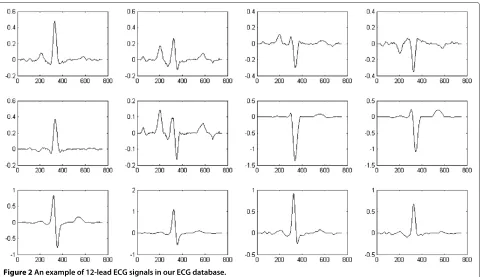
categories: the training set and the test set. We use the former to generate the projection tensors and train the SVM model. The models are then used for the classifica-tion of the testing dataset. We randomly split the original dataset into two subsets: the training set consists of 20,000 beats, and the 45,716 remaining beats are used for testing. The ratio are 1:3 and 2:3 of the total data for the train-ing and testtrain-ing sets, respectively. The size of the traintrain-ing set and of the testing set for each specific type are listed in Table 1. Figure 2 presents an example of a 12-lead ECG signal found in our database. In the experiment, the set is randomly split; the listed result is an average over several experiments.
11.2 Results on dataset
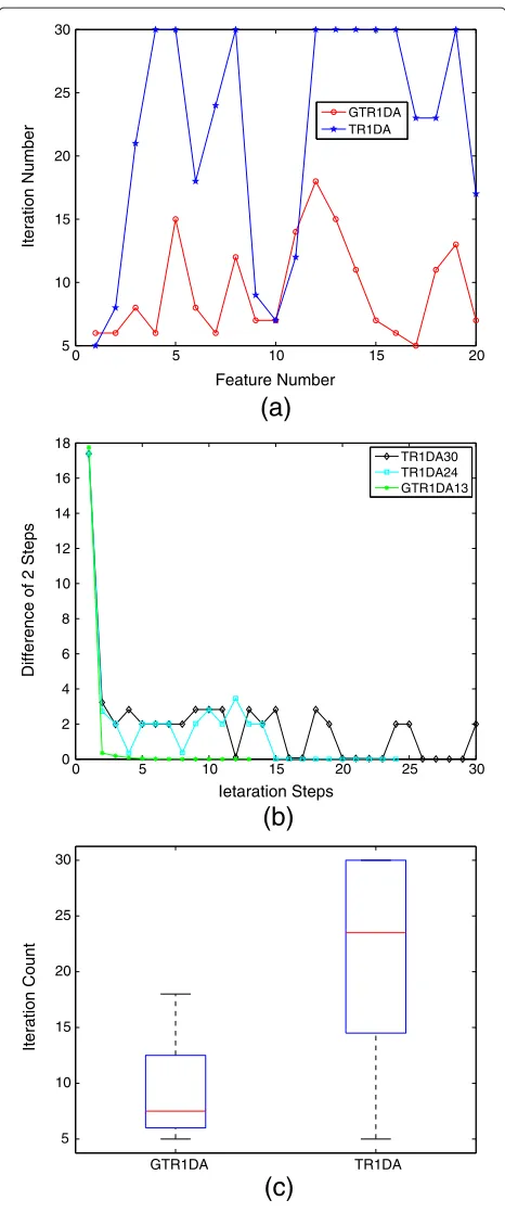
We first compare the convergence of TR1DA to our extended version GTR1DA. The result is shown in Figure 3a. Note that the pattern shape of the two methods look alike; the same observation also applies to the shape of the curves. For the feature of the 5th, 8th, 12th, and 19th dimension, both GTR1DA and TR1DA need more iter-ation steps. However, by comparing the two methods, it is obvious that GTR1DA needs less steps to convergence than the original TR1DA method. Overall, the number of iterations required by our new method is about 1:3 of the original TR1DA. In our experiments, the iteration count threshold was fixed to 30. Therefore, when the iter-ation count reaches 30, in the TR1DA case, it may indicate that the algorithm did not converge. In fact, during the
0 5 10 15 20 5
10 15 20 25 30
Feature Number
Iteration Number
GTR1DA TR1DA
(a)
0 5 10 15 20 25 30
0 2 4 6 8 10 12 14 16 18
Ietaration Steps
Difference of 2 Steps
TR1DA30 TR1DA24 GTR1DA13
(b)
GTR1DA TR1DA
5 10 15 20 25 30
Iteration Count
(c)
Figure 3Comparison of the convergence condition of GTR1DA and TR1DA.(a)Iteration number of each dimension,(b)converge process of GTR1DA and TR1DA (number behind the method name is the iteration count), and(c)iteration count statistics.
experiment, if TR1DA does not converge within 30 steps, it iterates with a small gap and, in most cases, cannot converge even with more steps.
On Figure 3b, the Frobenius norm of the difference of a two-step projection tensor is shown. GTR1DA appears to converge very fast and very smoothly, without any fluc-tuations or sudden increase in the process. It remains substantially and monotonically decreasing; on the con-trary, TR1DA starts fluctuating after a few steps. Despite this behavior, it sometimes achieves good convergence, although it always requires more iteration steps than GTR1DA. It can also happen that TR1DA fails to converge after 30 iterations while only fluctuating in a very small range. The number following the method name in the dia-gram represents the total number of iterations. Figure 3c shows a statistics of the iteration count of GTR1DA and TR1DA. GTR1DA displays an evident advantage over TR1DA.
In addition, since both TR1DA and GTR1DA are tensor learning approaches, the selection of a proper initial value has a great impact on the convergence of the algorithm. Figure 4 shows the improvement brought by our optimal initial value selection method. It compares the number of iterations when run with a random initial value and with our optimal initial value. The difference in the final result is quite large as in the random case. The number of itera-tions fluctuates between four and seven, against three and four using our optimal initial value.
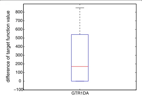
Figure 4 shows how important a proper choice for the initial value is. Indeed, it not only improves the conver-gence speed but also decreases the number of iterations, leading to a much higher computational efficiency. The iteration step count is more stable: fluctuating less and displaying only small variations. Figure 5 shows the time cost of calculating the initial value. Actually, a good ini-tial value sometimes leads to a better solution. Here, we compare the target function value of the calculated initial value and the random initial value in Figure 6. Sometimes, the calculated initial value leads to a better solution.
Randon_Initial_Value Calculated_Initial_Value 2
3 4 5 6 7 8
Iteration Number
GTR1DA 550
600 650 700 750 800 850 900 950
Time cost(s)
Figure 5Time cost of calculating the initial value.
In GTR1DA, we consider the closing points of differ-ent classes to calculate the optimal projection tensor. In fact, choosing an optimal proportion requires a trade-off between efficiency and effectiveness. A lower proportion leads to a higher efficiency as in Figure 7, but at the same time, the effectiveness follows a curve which depends on the point proportion. Therefore, using either a too-high or a too-low proportion can lower the classification accuracy. Table 2 compares the classification accuracy for differ-ent point proportions. It lists each class accuracy and aver-age accuracy for the followingm% values in Equation 19: 0.5%, 1.2%, 1.5%, 5.5%, and 8%. To prevent the overlapping point pairs, then% is set with 0.2%. Through this compar-ison, we observe that the 1.2% proportion results in the highest classification accuracy.
On the other hand, the proportion can greatly influ-ence the time cost. Figure 7 compares the time cost of one loop for the proportions 0.5%, 1.2%, 1.5%, 5.5%, and 8%. It is clear on the figure that a higher proportion implies a
GTR1DA −100
0 100 200 300 400 500 600 700 800
difference of target function value
Figure 6The target function value difference.Calculated initial value target function value minus random initial value target function value.
8% 5.5% 1.5% 1.2% 0.5%
0 500 1000 1500
Time Cost of One Loop(s)
Figure 7Single-loop time cost of different closing point proportions.
higher time cost and greater fluctuations and variations. One loop using 8% takes from 1,200 to 1,500 s, while with 5.5%, it is between 800 and 1,000 s. It even drops down to 120, 50, and 20 s for 1.5% 1.2%, and 0.5%, respectively. As the fluctuations in the latter two cases remain small, we need to reduce the proportion of the points as much as possible in order to improve the computational efficiency while maintaining a high classification accuracy.
Figure 8 shows the convergence process with respect to the time cost. Figure 9 represents the statistics of a one-feature calculation time. In this case, the closing point proportion is 1.2%. Also, note that the time cost remains acceptable compared to that in TR1DA.
As for the ECG signal processing, the most important is the classification accuracy. Therefore, we compared the following different methods over the dimensions 1 to 20 in Figure 10: GTR1DA, TR1DA, UMPCA, PCA, ICA, LDA, and regularized LDA. As for rLDA, PCA, ICA, and LDA, the tensor data is first expanded into a vector, and then the projection vectors are calculated based on the vectorized data. Finally, the top 20 projection vectors are selected to calculate the features exploited in the classification.
Figure 10 highlights the superiority of the tensor-based approach over the vector space-based methods. The main reason is that tensor-based approaches take the tensor
Table 2 Classification accuracy of different closing points proportion
Percentage (%) N L R V S E Average
8 97.34 96.80 97.65 96.30 97.47 97.67 97.21
5.5 98.45 97.67 99.20 97.56 97.26 98.47 98.10
1.5 99.11 98.53 100.00 99.60 99.90 99.60 99.46
1.2 99.86 99.73 100.00 100.00 100.00 100.00 99.93
0 500 1000 1500 2000 2500 0
2 4 6 8 10 12 14 16 18
Time cost(s)
Difference of 2 Steps
TR1DA30 TR1DA24 GTR1DA13
Figure 8Converge process of GTR1DA and TR1DA while calculating one projection tensor with time cost.
data directly as input, preventing SSS problem [7]. More-over, it enables the utilization of the structural informa-tion in the tensor data. The original TR1DA displays a higher classification accuracy under low dimension conditions; however, for higher dimensions, GTR1DA outperforms TR1DA. Both perform better than UMPCA though. As for the vector space methods, from the best to the worst, they are classified as follows for the lower dimension case: LDA, rLDA, PCA, and ICA. They are classified as follows for higher dimensions: PCA, rLDA, ICA, and LDA. ICA displays a sudden accuracy increase after dimension 15.
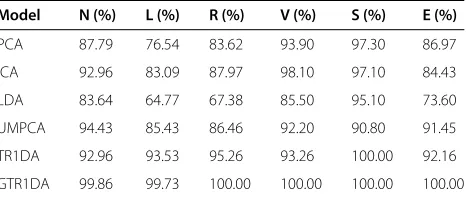
Table 3 presents a clear comparison of the differ-ent methods depending on the classification accuracy of each class. It is obvious that TR1DA and GTR1DA have higher accuracy and outperform the others. In addition, our method GTR1DA performs better than the original TR1DA. Four classes of ECG have a 100% accuracy, so it is obvious that our extension impacts the experiments.
GTR1DA TR1DA
1500 1600 1700 1800 1900 2000
Time cost(s)
Figure 9Total time cost of calculating one projection tensor comparison between GTR1DA and TR1DA.
0 5 10 15 20
30 % 40 % 50 % 60 % 70 % 80 % 90 % 100%
Feature Dimensions
Classification accuracy
PCA ICA LDA rLDA UMPCA TR1DA GTR1DA
Figure 10Classification accuracy of different approaches with different feature dimensions.
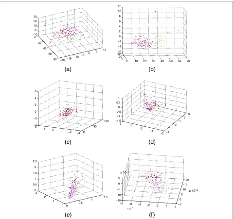
To further illustrate the effectiveness of our approach and show a clear illustration of better class separation, we extract three dimension features of three classes using some feature extraction methods and plot their 3D distri-bution (Figure 11).
In Figure 11, it is clear that GTR1DA, TR1DA, and LDA display cluster characteristics. This is to be con-trasted by other methods such as PCA, ICA, and UMPCA. Both LDA and TR1DA seem to display a better cluster characteristic; however, there is an obvious overlap at the boundary of each two classes. Our method calculates the projection tensors based on the data distribution near-ing the boundary of each two classes. That explains why we achieve an almost 100% accuracy. Hence, in the end, GTR1DA features a better classification accuracy than the other two methods.
To analyze the performance of our approach, we com-pare the classification accuracy of the wavelet transform approach [1], of the neural networks approach for deter-mining the features of a given ECG signal [2], of the active learning method [3], and of GTR1DA. The results are shown in Table 4. Our method clearly displays an advantage over all the other methods.
Table 3 Comparison of different approaches’ classification accuracy
Model N (%) L (%) R (%) V (%) S (%) E (%)
PCA 87.79 76.54 83.62 93.90 97.30 86.97
ICA 92.96 83.09 87.97 98.10 97.10 84.43
LDA 83.64 64.77 67.38 85.50 95.10 73.60
UMPCA 94.43 85.43 86.46 92.20 90.80 91.45
TR1DA 92.96 93.53 95.26 93.26 100.00 92.16
0
20
40
60
80 −20 −15 −10 −5
0 5
10 −10
0 10 20 30
(a)
0 10 20 30 40 50 60 70
0 20 40−6 −4 −2 0 2 4 6 8 10 12
(b)
0 50
100
−4 −2 0 2 4 6 −4 −2 0 2 4 6
(c)
−2 −1
0 1
2 3
−2 −1 0 1 2 −1.5 −1 −0.5 0 0.5 1
(d)
0 0.5
1 1.5
0 1 2 3 0 0.5 1 1.5 2 2.5
(e)
−8 −6 −4 −2 0 2 4
x 10−3
−5 0 5
10 15
20
x 10−3
−15 −10 −5 0 5
x 10−3
(f)
Figure 113D Distribution of extracted three dimension features.(a)GTR1DA,(b)TR1DA,(c)UMPCA,(d)PCA,(e)ICA, and(f)LDA.
Table 4 Comparison of our approach with other state-of-the-art ECG classification methods
Model N (%) L (%) R (%) V (%) S (%) E (%)
Wavelet 97.86 93.67 91.89 94.75 92.74 95.79
Neural 94.68 95.37 92.57 96.58 98.54 99.73
networks
Active 93.36 94.49 89.47 96.37 91.63 92.47
learning
GTR1DA 99.86 99.73 100.00 100.00 100.00 100.00
12 Conclusions
between-class scatter matrix problem by considering the distribution of closing points near the boundary of the various classes. To improve the calculation speed and sta-bility, an optimal calculation method for tensor learning approaches was also proposed to compute an optimal ini-tial value. The results of the experiment showed that our new tensor-based scheme outperforms traditional vector-based methods. In addition, classification is much more accurate when using GTR1DA than when using the orig-inal TR1DA and UMPCA methods. The experiment also shows a critical performance improvement caused by a judicious choice of the initial value. This indicates that GTR1DA, and tensor-based schemes in general, are well fitted, effective, and robust data exploration tools for clas-sifying 12-lead ECG signals.
Endnote
a We will make the ECG data public. Please see the
website http://bcmi.sjtu.edu.cn/ehealth/.
Competing interests
The authors declares that they have no competing interests.
Acknowledgements
The work was supported by the National Natural Science Foundation of China (grant nos. 91120305 and 61272251).
Received: 29 June 2013 Accepted: 26 December 2013 Published: 14 January 2014
References
1. Q Zhao, L Zhang, ECG feature extraction and classification using wavelet transform and support vector machines, in2005 International Conference on Neural Networks and Brain(IEEE, Piscataway, 2005), pp. 1089–1092 2. Y-R Hwang, K-K Jen, ECG feature extraction and classification using
cepstrum and neural networks. J. Med. Biol. Eng.28(1), 31 (2008) 3. E Pasolli, F Melgani, Active learning methods for electrocardiographic
signal classification. IEEE Trans. Inf. Technol. Biomed.14(6), 1405–1416 (2010)
4. H Zhang, L Zhang, ECG analysis based on PCA and support vector machines. International Conference on Neural Networks and Brain 2, 743–747 (2005)
5. Y Wu, L Zhang, ECG classification using ICA features and support vector machines, inICONIP (1), ed. by Lu B L, Zhang L, and Kwok J T. Lecture notes in Computer Science, vol. 7062 (Springer, Heidelberg, 2011), pp. 146–154
6. K Huang, L Zhang, Y Wu, ECG classification based on non-cardiology feature, inProceedings of the 9th international conference on Advances in Neural Networks - volume part II, ISNN’12(Springer, Heidelberg, 2012), pp. 179–186
7. Y He, Solving undersampled problem of lDA using Gram-Schmidt orthogonalization procedure in difference space, inProceedings of the 2009 International Conference on Advanced Computer Control,Washington DC (IEEE Computer Society, Piscataway, 2009), pp. 153–157
8. J Li, L Zhang, D Tao, H Sun, Q Zhao, A prior neurophysiologic knowledge free tensor-based scheme for single trial eeg classification. IEEE Trans. Neural Syst. Rehabil. Eng.17(2), 107–115 (2009)
9. D Tao, X Li, X Wu, SJ Maybank, General tensor discriminant analysis and Gabor features for gait recognition. IEEE Trans. Pattern Anal. Mach. Intell. 29(10), 1700–1715 (2007)
10. H Lu, KN Plataniotis, AN Venetsanopoulos, Multilinear principal component analysis of tensor objects for recognition, inProc. Int. Conf. on Pattern Recognition2, (2006), pp. 776–779
11. H Lu, KN Plataniotis, AN Venetsanopoulos, MPCA: multilinear principal component analysis of tensor objects. IEEE Trans. Neural Netw.19(1), 18–39 (2008)
12. H Lu, KN Plataniotis, AN Venetsanopoulos, Uncorrelated multilinear principal component analysis through successive variance maximization, in25th International Conference on Machine Learning (ICML)(Helsinki, 2008) 13. H Lu, KN Plataniotis, AN Venetsanopoulos, Uncorrelated multilinear
principal component analysis for unsupervised multilinear subspace learning. IEEE Transactions on Neural Networks20(11), 1820–1836 (2009) 14. D Tao, X Li, X Wu, S Maybank, Tensor rank one discriminant analysis-a
convergent method for discriminative multilinear subspace selection. Neurocomput.71(10–12), 1866–1882 (2008)
15. H Lu, KN Plataniotis, AN Venetsanopoulos, A survey of multilinear subspace learning for tensor data. Pattern Recognit.44(7), 1540–1551 (2011)
16. JB Allen, LR Rabiner, A unified approach to short-time Fourier analysis and synthesis. Proc. IEEE65(11), 1558–1564 (1977)
17. Y Panagakis, C Kotropoulos, GR Arce, Non-negative multilinear principal component analysis of auditory temporal modulations for music genre classification. Trans. Audio, Speech Lang. Proc.18(3), 576–588 (2010) 18. F Miwakeichi, PA Valdes-Sosa, E Aubert-Vazquez, JB Bayard, J Watanabe,
H Mizuhara, Y Yamaguchi, Decomposing EEG data into
space-time-frequency components using parallel factor analysis and its relation with cerebral blood flow, inNeural Information Processing
(Springer, Heidelberg, 2008), pp. 802–810
19. M De Vos, A Vergult, L De Lathauwer, W De Clercq, S Van Huffel, P Dupont, A Palmini, W Van Paesschen, Canonical decomposition of ictal scalp {EEG} reliably detects the seizure onset zone. NeuroImage. 37(3), 844–854 (2007)
20. E Acar, C Aykut-Bingol, H Bingol, R Bro, B Yener, Multiway analysis of epilepsy tensors, inProceedings 15th International Conference on Intelligent Systems for Molecular Biology (ISMB) 6th European Conference on Computational Biology (ECCB), Vienna, Austria, July 21–25, 2007(Oxford University Press, Oxford, 2007), pp. 10–18
21. F Song, D Zhang, D Mei, Z Guo, A multiple maximum scatter difference discriminant criterion for facial feature extraction. IEEE Trans. Syst. Man Cybern Part B37(6), 1599–1606 (2007)
22. J Gao L Xiang, Laplacian maximum scatter difference discriminant criterion. ICAIC224(1), 691–697 (2011)
23. JM Leiva-Murillo, A Artés-Rodríguez, Maximization of mutual information for supervised linear feature extraction. IEEE Trans. Neural Netw.18(5), 1433–1441 (2007)
24. C Dhir, S Lee, Discriminant independent component analysis, inIntelligent Data Engineering and Automated Learning - IDEAL 2009, ed. by E Corchado, H Yin. Lecture Notes in Computer Science, vol. 5788 (Springer,
Heidelberg, 2009), pp. 219–225
25. G Takács, D Tikk, Alternating least squares for personalized ranking, in
Proceedings of the Sixth ACM Conference on Recommender Systems, RecSys ’12(ACM, New York, 2012), pp. 83–90
26. E Acar, TG Kolda, DM Dunlavy, An optimization approach for fitting canonical tensor decompositions. Technical report, Sandia National Laboratories (2009)
27. TG Kolda, BW Bader, Tensor decompositions and applications. SIAM Rev. 51(3), 455–500 (2009)
28. CM Bishop,Pattern Recognition and Machine Learning,1st edn. (Springer, Heidelberg, 2006)
29. CW Hsu, CC Chang, CJ Lin.A Practical Guide to Support Vector Classification,
Technical report, National Taiwan University (2000)
doi:10.1186/1687-6180-2014-2