Vector Processor- A Study
Achin Pal ;Tanya Sharma; Sumit Kumar Das
Computer science and engineering department, MDU Rohtak, India
ABSTRACT
The power of vector processors comes from their ability to process several elements at once (applying the same operations to all elements in a short vector). This, combined with the standard processor techniques of independent processing units (load/store, integer, float, vector) running in parallel, and pipelined units processing several instructions simultaneously (sequentially up to the instruction latency) make it possible to process multiple data elements per clock cycle. Achieving this in practice is far from easy and requires an in-depth knowledge of the processor and a detailed analysis and understanding of the algorithm. For large datasets memory management is also an issue: a processor waiting for data is not producing results. This paper deals with history and examples of vector processors and also helps to enlighten about the concept of VECTOR PROCESSOR.
1)
INTRODUCTION
A vector processor is a processor that can operate on entire vectors with one instruction, i.e. the operands of some instructions specify complete vectors. For example, consider the following add instruction:
C = A + B
In both scalar and vector machines this means ``add the contents of A to the contents of B and put the sum in C.'' In a scalar machine the operands are numbers, but in vector processors the operands are vectors and the instruction directs the machine to compute the pairwise sum of each pair of vector elements. A processor register, usually called the vector length register, tells the processor how many individual additions to perform when it adds the vectors.
A vectorizing compiler is a compiler that will try to recognize when loops can be transformed into single
vector instructions. For example, the following loop can be executed by a single instruction on a vector processor:
DO 10 I=1,N A(I) = B(I) + C(I) 10 CONTINUE
This code would be translated into an instruction that would set the vector length to N followed by a vector add instruction.
The use of vector instructions pays off in two different ways. First, the machine has to fetch and decode far fewer instructions, so the control unit overhead is greatly reduced and the memory bandwidth necessary to perform this sequence of operations is reduced a corresponding amount. The second payoff, equally important, is that the instruction provides the processor with a regular source of data. When the vector instruction is initiated, the machine knows it will have to fetch pairs of operands which are arranged in a regular pattern in memory. Thus the processor can tell the memory system to start sending those pairs. With an interleaved memory, the pairs will arrive at a rate of one per cycle, at which point they can be routed directly to a pipelined data unit for processing. Without an interleaved memory or some other way of providing operands at a high rate the advantages of processing an entire vector with a single instruction would be greatly reduced.
operands from the vector registers and returning the
results to a vector register.
The advantage of memory to memory machines is the ability to process very long vectors, whereas register to register machines must break long vectors into fixed length segments. Unfortunately, this flexibility is offset by a relatively large overhead known as the startup time, which is the time between the initialization of the instruction and the time the first result emerges from the pipeline. The long startup time on a memory to memory machine is a function of memory latency, which is longer than the time it takes to access a value in an internal register. Once the pipeline is full, however, a result is produced every cycle or perhaps every other cycle. Thus a performance model for a vector processor is of the form
where is the startup time, is the length of the vector and is an instruction dependent constant,
usually , 1 or 2.
Examples of this type of architecture include the Texas Instruments Inc. Advanced Scientific Computer and a family of machines built by Control Data Corp. known first as the Cyber 200 series and later the ETA-10 when Control Data Corp. founded a separate company known as ETA Systems Inc. These machines appeared in the mid-1970s after a long development cycle that left them with dated technology and disappeared in the mid-1980s. For a thorough discussion of their characteristics, see Hockney and Jesshope. One of the major reasons for their demise was the large startup time, which was on the order of 100 processor cycles. This meant that short vector operations were very inefficient, and even for vectors of length 100 the machines were delivering only about half their maximum performance. In a later section we will see how this vector length that yields half of peak performance is used to characterize vector computers.
In the register to register machines the vectors have a relatively short length, 64 in the case of the Cray family, but the startup time is far less than on the memory to memory machines. Thus these machines are much more efficient for operations involving short vectors, but for long vector operations the vector registers must loaded with each segment
before the operation can continue. Register to register machines now dominate the vector computer market, with a number of offerings from Cray Research Inc., including the Y-MP and the C-90. The approach is also the basis for machines from Fujitsu, Hitachi and NEC. Clock cycles on modern vector processors range from 2.5ns (NEC SX-3) to 4.2ns (Cray C90), and single processor performance on LINPACK benchmarks is in the range of 1000 to 2000 MFLOPS (1 to 2 GFLOPS).
The basic processor architecture of the Cray supercomputers has changed little since the Cray-1 was introduced in 1976. There are 8 vector registers, named V0 through V7, which each hold 64 64-bit words. There are also 8 scalar registers, which hold single 64-bit words, and 8 address registers (for pointers) that have 20-bit words. Instead of a cache, these machines have a set of backup registers for the scalar and address registers; transfer to and from the backup registers is done under program control, rather than by lower level hardware using dynamic memory referencing patterns.
The original Cray-1 had 12 pipelined data processing units; newer Cray systems have 14. There are separate pipelines for addition, multiplication,
computing reciprocals (to divide by , a Cray
computes ), and logical operations. The cycle time of the data processing pipelines is carefully matched to the memory cycle times. The memory system delivers one value per clock cycle through the use of 4-way interleaved memory.
An interesting feature introduced in the Cray computers is the notion of vector chaining. Consider the following two vector instructions:
V2 = V0 * V1 V4 = V2 + V3
and routed to the pipeline. This situation is shown in
Figure 16, where the operands from V0 and V1 that are currently in the multiplier pipeline are indicated by gray cells. At this point, the system is fetching V0[k] and V1[k] to route them to the first stage of the pipeline and V2[j] is just leaving the pipeline. Vector chaining relies on the path marked with an asterisk. While V2[j] is being stored in the vector register, it is also routed directly to the pipelined adder, where it is matched with V3[j]. As the figure shows, the second instruction can begin even before the first finished, and while both are executing the machine is producing two results per cycle (V4[i] and V2[j]) instead of just one.
Without vector chaining, the peak performance of the Cray-1 would have been 80 MFLOPS (one full pipeline producing a result every 12.5ns, or 80,000,000 results per second). With three pipelines chained together, there is a very short burst of time where all three are producing results, for a theoretical peak performance of 240 MFLOPS. In principle vector chaining could be implemented in a memory-to-memory vector processor, but it would require much higher memory bandwidth to do so. Without chaining, three ``channels'' must be used to fetch two input operand streams and store one result stream; with chaining, five channels would be needed for three inputs and two outputs. Thus the ability to chain operations together to double performance gave register- to-register designs another competitive edge over memory-to- memory designs.
2)
HISTORY
2.1) EARLY WORK
Vector processing development began in the early 1960s at Westinghouse in their Solomon project. Solomon's goal was to dramatically increase math performance by using a large number of simple math co-processors under the control of a single master CPU. The CPU fed a single common instruction to all of the arithmetic logic units (ALUs), one per "cycle", but with a different data point for each one to work on. This allowed the Solomon machine to apply a single algorithm to a large data set, fed in the form of an array.
In 1962, Westinghouse cancelled the project, but the effort was restarted at the University of Illinois as the ILLIAC IV. Their version of the design originally
called for a 1 GFLOPS machine with 256 ALUs, but, when it was finally delivered in 1972, it had only 64 ALUs and could reach only 100 to 150 MFLOPS. Nevertheless it showed that the basic concept was sound, and, when used on data-intensive applications, such as computational fluid dynamics, the "failed" ILLIAC was the fastest machine in the world. The ILLIAC approach of using separate ALUs for each data element is not common to later designs, and is often referred to under a separate category, massively parallel computing.
2.2)SUPERCOMPUTERS
The first successful implementation of vector processing appears to be the Control Data CorporationSTAR-100 and the Texas InstrumentsAdvanced Scientific Computer (ASC). The basic ASC (i.e., "one pipe") ALU used a pipeline architecture that supported both scalar and vector computations, with peak performance reaching approximately 20 MFLOPS, readily achieved when processing long vectors. Expanded ALU configurations supported "two pipes" or "four pipes" with a corresponding 2X or 4X performance gain. Memory bandwidth was sufficient to support these expanded modes. The STAR was otherwise slower than CDC's own supercomputers like the CDC 7600, but at data related tasks they could keep up while being much smaller and less expensive. However the machine also took considerable time decoding the vector instructions and getting ready to run the process, so it required very specific data sets to work on before it actually sped anything up.
Other examples followed. Control Data Corporation
tried to re-enter the high-end market again with its ETA-10 machine, but it sold poorly and they took that as an opportunity to leave the supercomputing field entirely. In the early and mid-1980s Japanese companies (Fujitsu, Hitachi and Nippon Electric Corporation (NEC) introduced register-based vector machines similar to the Cray-1, typically being slightly faster and much smaller. Oregon-based Floating Point Systems (FPS) built add-on array processors for minicomputers, later building their own mini-supercomputers. However Cray continued to be the performance leader, continually beating the competition with a series of machines that led to the Cray-2, Cray X-MP and Cray Y-MP. Since then, the supercomputer market has focused much more on massively parallel processing rather than better implementations of vector processors. However, recognizing the benefits of vector processing IBM developed Virtual Vector Architecture for use in supercomputers coupling several scalar processors to act as a vector processor.
2.3) SIMD
Vector processing techniques have since been added to almost all modern CPU designs, although they are typically referred to as SIMD. In these implementations, the vector unit runs beside the main scalarCPU, and is fed data from vector instruction aware programs.
3)
ARCHITECTURE
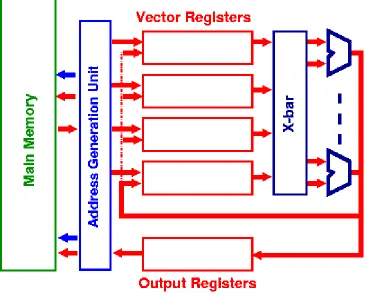
Commonly called supercomputers, the vector processors are machines built primarily to handle large scientific and engineering calculations. Their performance derives from a heavily pipelined architecture which operations on vectors and matrices can efficiently exploit.
Data is read into the vector registers which are FIFO
queues capable of holding 50-100 floating point values. A machine will be provided with several vector registers, Va, Vb, etc. The instruction set will contain instruction which:
load a vector register from a location in memory,
perform operations on elements in the vector registers and
store data back into memory from the vector registers.
4)
DESCRIPTION
In general terms, CPUs are able to manipulate one or two pieces of data at a time. For instance, most CPUs have an instruction that essentially says "add A to B and put the result in C". The data for A, B and C could be—in theory at least—encoded directly into the instruction. However, in efficient implementation things are rarely that simple. The data is rarely sent in raw form, and is instead "pointed to" by passing in an address to a memory location that holds the data. Decoding this address and getting the data out of the memory takes some time, during which the CPU traditionally would sit idle waiting for the requested data to show up. As CPU speeds have increased, this memory latency has historically become a large impediment to performance; see Memory wall.
In order to reduce the amount of time consumed by these steps, most modern CPUs use a technique known as instruction pipelining in which the
instructions pass through several sub-units in turn. The first sub-unit reads the address and decodes it, the next "fetches" the values at those addresses, and the next does the math itself. With pipelining the "trick" is to start decoding the next instruction even before the first has left the CPU, in the fashion of an assembly line, so the address decoder is constantly in use. Any particular instruction takes the same amount of time to complete, a time known as the latency, but the CPU can process an entire batch of operations much faster and more efficiently than if it did so one at a time.
Vector processors take this concept one step further. Instead of pipelining just the instructions, they also pipeline the data itself. The processor is fed instructions that say not just to add A to B, but to add all of the numbers "from here to here" to all of the numbers "from there to there". Instead of constantly having to decode instructions and then fetch the data needed to complete them, the processor reads a single instruction from memory, and it is simply implied in the definition of the instruction itself that the instruction will operate again on another item of data, at an address one increment larger than the last. This allows for significant savings in decoding time.
5)
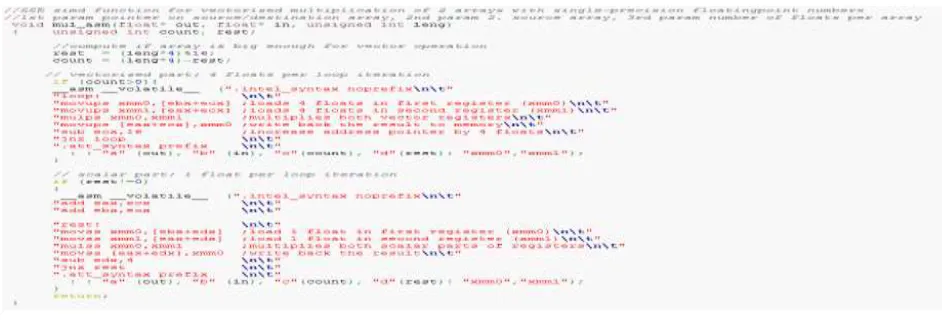
REAL WORLD EXAMPLE
Shown below is an actual x86 architecture example for vector instruction usage with the SSE instruction set. The example multiplies two arrays of single precision floating point numbers. It's written in the C language with inline assembly code parts for compilation with GCC (32bit).
SUMMARY
A vector processor, or array processor, is a central processing unit (CPU) that implements an instruction set containing instructions that operate on one-dimensional arrays of data called vectors. This is in contrast to a scalar processor, whose instructions operate on single data items. Vector processors can greatly improve performance on certain workloads, notably numerical simulation and similar tasks. Vector machines appeared in the early 1970s and dominated supercomputer design through the 1970s into the 90s, notably the various Cray platforms. The rapid fall in the price-to-performance ratio of conventional microprocessor designs led to the vector supercomputer's demise in the later 1990s.
Today, most commodity CPUs implement architectures that feature instructions for a form of vector processing on multiple (vectorized) data sets, typically known as SIMD (Single Instruction, Multiple Data). Common examples include VIS, MMX, SSE, AltiVec and AVX. Vector processing techniques are also found in video game console hardware and graphics accelerators. In 2000, IBM, Toshiba and Sony collaborated to create the Cell processor, consisting of one scalar processor and eight vector processors, which found use in the Sony PlayStation 3 among other applications.
Other CPU designs may include some multiple instructions for vector processing on multiple (vectorised) data sets, typically known as MIMD (Multiple Instruction, Multiple Data) and realized with VLIW. Such designs are usually dedicated to a particular application and not commonly marketed for general purpose computing. In the FujitsuFR-V VLIW/vector processor both technologies are combined.
DISCLOSURE STATEMENT
There is no financial support for this research work from the funding agency.
ACKNOWLEDGMENTS
We thank our guide for his timely help, giving outstanding ideas and encouragement to finish this research work successfully.
SIDE BAR
Comparison:
it is an act of assessment or evaluation of things side by side in order to see to what extent they are similar or different. It is used to bring out similarities or differences between two things of same type mostly to discover essential features or meaning either scientifically or otherwise.Content:
The amount of things contained in something. Things written or spoken in a book, an article, a programme, a speech, etc.DEFINITION
Latency- it is a time interval between the stimulation and response, or, from a more general point of view, as a time delay between the cause and the effect of some physical change in the system being observed.
Referencing- provide (a book or article) with citations of sources of information.
Dynamic- characterized by constant change,
activity, or progress.
Dominate- be the most important or
conspicuous person or thing in.
REFERENCES
http://www.nasoftware.co.uk/home/index.php/ser vices/vector-processors
https://www.cs.auckland.ac.nz/~jmor159/363/ht ml/vector.html
http://www.phy.ornl.gov/csep/ca/node24.html
http://en.wikipedia.org/wiki/Vector_processor
REALATED REFERNCES
[1.] Malinovsky, B.N. (1995 (see also here http://www.sigcis.org/files/SIGCISMC2010_001.pdf and english version here)). The history of computer technology in their faces (in Russian). Kiew: Firm "KIT". ISBN 5-7707-6131-8. Check date values in: |date= (help)
[2.] Kunzman, D. M.; Kale, L. V. (2011). "Programming Heterogeneous Systems". "2011 IEEE International Symposium on Parallel and Distributed Processing Workshops and Phd Forum". p. 2061. doi:10.1109/IPDPS.2011.377. ISBN 978-1-61284-425-1. edit