Article
1
Mathematical Analysis of Transfusion—Transmitted
2
Malaria Model with Optimal Control
3
Michael Olaniyi Adeniyi * and Oluwaseun Raphael Aderele
4
Department of Mathematics and Statistics, School of Pure and Applied Sciences, Lagos State Polytechnic,
5
Ikorodu, Lagos State, Nigeria; [email protected]
6
* Correspondence: [email protected]
7
8
Abstract: An SIRS (Susceptible–Infected–Removed-Susceptible) mathematical model for the
9
transmission dynamics of the Transfusion–Transmitted Malaria (TTM) model with optimal control
10
pair u1(t) and u2(t) was developed and studied in this research work. The model Transfusion–
11
Transmitted Malaria disease–free equilibrium and endemic equilibriums points were determined.
12
The model exhibited two equilibriums; disease-free and endemic equilibrium. It is shown that the
13
disease–free equilibrium was locally asymptotically stable if the associated basic reproduction
14
numbers R0 is less than unity while the disease persists if
R
0 is greater than unity. The global15
stability of the Transfusion–Transmitted Malaria model at the disease-free equilibrium was
16
established using the comparison method. The optimality system was derived and an optimal
17
control model of blood screening and drug treatment for the Transfusion–Transmitted Malaria
18
model was investigated. Conditions for the optimal control were considered using Pontryagin’s
19
Maximum Principle and solved numerically using the Forward and Backward Finite Difference
20
Method (FBDM). Numerical results obtained are in perfect agreement with our analytical results.
21
Keywords: malaria; transfusion–transmitted; basic reproduction number; stability; equilibrium;
22
optimal control
23
24
1. Introduction
25
Transfusion–transmitted malaria (TTM) was first documented in 1911 [5]. The global incidence
26
and occurrence of TTM based on available data indicates that over hundred cases are reported
27
annually, mostly restricted to endemic countries [2]. The chances of TTM due to donor blood in Sub
28
Saharan African countries is increased due to malaria prevalence in donor blood sample [8]. In
29
countries where malaria is endemic, differentiating cases of TTM from natural infection still remain
30
a challenge as malaria infection occurrence after transfusion may be as a result of either natural
31
infection (infection through bites from an infected female anopheles mosquito) or transfusion
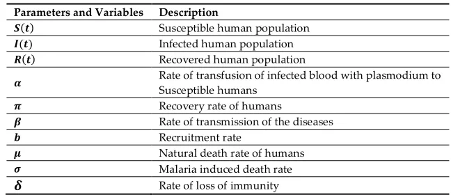
32
transmitted (TT). This explains the reason the number of TTM cases in endemic countries is
33
under-reported. Acquisition of malaria parasite due to donor exposure is an increasing problem as a
34
result in global travelling and immigration. Thus, it is more challenging to develop an optimal
35
strategy to reduce the risk of TTM in endemic countries without unnecessary exclusion of blood
36
donation which remain a subject of debate. In [10,11], a general overview of current strategies in
37
non-endemic countries was considered. The strict donor deferral system which is based on travel
38
history of individual has been adopted by most countries, However, this strategy is not optimal due
39
to many healthy donors are differed which may result in donation loss because lengthy deferrals
40
may discourage the donors from coming back [5]. Consequently, the optimal control strategy for a
41
given country or location may vary according to the background level of malaria risk faced by the
42
donor and the recipient population viz-a-viz the resources available. Thus, we aim to study in this
43
work mathematical analysis of transfusion–transmitted malaria TTM) model with optimal control
44
2. Model Formation
45
We formulate the mathematical model for the Transfusion–Transmitted Malaria by considering
46
the dynamical system of equation with optimal control analysis for human population only. The
47
human population is divided into three sub-groups: Susceptible S(t)-Infected (I(t)) –Removal (R(t)).
48
Thus, we assume that the total populations of humans is N(t) = S(t)+I(t)=R(t). Individual are recruited
49
into the population at rate b and die naturally at rate
. Recovered humans become susceptible50
again due to loss of immunity at rate . Our model also includes the rate of transfusion of infected
51
blood and transmitted rate of the disease with malaria induced death rate.
52
For our dynamical equations, we define the following variables and parameters as follows:
53
Table 1. Description of variables and parameters of the model.
54
Parameters and Variables Description
( ) Susceptible human population
( ) Infected human population
( ) Recovered human population
Rate of transfusion of infected blood with plasmodium to Susceptible humans
Recovery rate of humans
Rate of transmission of the diseases Recruitment rate
Natural death rate of humans Malaria induced death rate Rate of loss of immunity
The dynamical equations for the transfusion–transmitted malaria model are given as follows:
55
(1)
With the following assumptions:
56
(1) Both recruitment rate (b) and natural death rate for humans (
) is assumed to be equal57
(2) Transmission of the plasmodium is via transfusion of blood to blood contact of infected blood
58
with plasmodium to a susceptible individual
59
(3) Due to the assumption made in (2), the Vector population is excluded
60
(4) Susceptible individual become infected upon blood to blood contact of infected blood with
61
plasmodium
62
The flow diagram for the model is given in Figure 1:
63
64
) ( ) ( ) ( ) (
) ( ) (
) (
) ( ) ( ) (
) ( ) ( )
( ) ( ) ( ) ( ) (
t R t
I t R
t I t
N t I t S t I
t R t S t
N t I t S t bN t S
h h
h
h h
h h h
h h h
h h h
h
65
66
( ) ( )
( )
67
68
69
70
71
72
Figure 1. Flow-chart of the transfusion–transmitted malaria model showing movements amongst
73
susceptible, infected and recovered compartments.
74
3. Model Analysis
75
System (1) is resolved by non-dimensionalizing the variables as follow by setting:
76
)
(
)
(
)
(
,
)
(
)
(
)
(
,
)
(
)
(
)
(
t
N
t
R
t
R
t
N
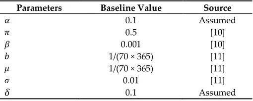
t
I
t
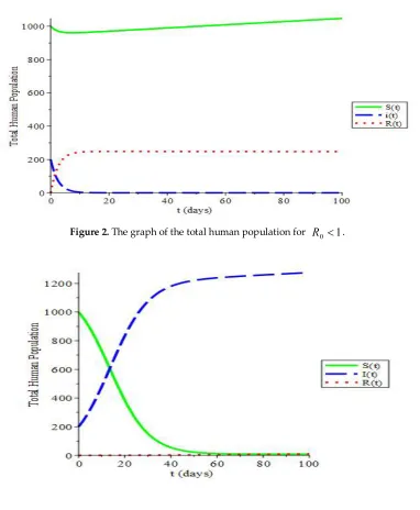
I
t
N
t
S
t
S
h h h h hh
(2))
(
)
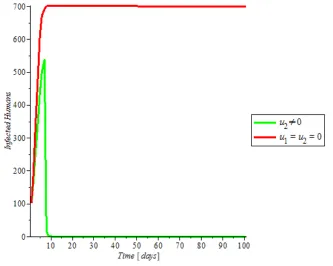
(
)
(
,
)
(
)
(
)
(
,
)
(
)
(
)
(
t
N
t
R
t
R
t
N
t
I
t
I
t
N
t
S
t
S
h h h h hh
(3)Substituting Equations (2) and (3) into (1) yields
77
)
(
)
(
)
(
)
(
)
(
)
(
)
(
)
(
)
(
)
(
)
(
)
(
)
(
)
(
t
R
t
I
t
R
t
I
t
S
t
I
t
I
t
R
t
S
t
S
t
I
b
t
S
(4)3.1. The Population Dynamics of the Model
78
Let
N
(
t
)
represent the total human population. Thus79
)
(
)
(
)
(
)
(
t
S
t
I
t
R
t
N
(5)Differentiating (5) with respect to t give
80
(
)
(
)
(
)
(
)
)
(
t
b
S
t
I
t
R
t
I
t
N
At disease free we obtain
81
( )
( )
N t
N t
b
(6)Since the recruitment rate (
b
) is equal to the natural death rate (
) and ast
, then the82
total human population reaches a value given as
83
b
t
N
(
)
(7)84
3.2. Positivity of Solution
85
For the Transfusion–Transmitted Malaria model of Equation (4) to be epidemiologically well
86
posed, we need to show that all solution with non-negative initial conditions will remain
87
non-negative, for all
t
0
.88
Theorem 3.1: Let: a R3 with
a (S(t),I(t),R(t)) R3:(S(t) I(t) R(t)) N(t) b ,
89
then the solution
(
S
(
t
),
I
(
t
),
R
(
t
)
)
of the system (4) are positive
t
0
.90
Proof: From the first differential equation of System (1),
91
dt
I
t
S
t
dS
t
S
I
dt
t
dS
)
(
)
(
)
(
)
(
Integrating both sides
92
tdt
t
I
t
S
t
dS
0)
(
)
(
)
(
To obtain93
t dt t Ike
t
S
0 ) ()
(
, at
t
0
)
(
)
0
(
K
S
t
S
, hence
.
0
,
0
)
0
(
)
(
0 ) (
t
e
S
t
S
t dt t I Similar reasoning can be used for other differential equations of Equation (4) hence, it follows
94
that the Transfusion–Transmitted Malaria model is positive and bounded with a unique solution.∎
95
3.3. The Local Stability of Disease-free Equilibrium,
P
096
System (4) has a disease-free equilibrium (DFE) obtained by setting the right-hand side of
97
Equation (4) to zero, given by
98
,
0
,
0
)
,
,
(
:
0
b
R
I
S
P
(8)The Jacobian Matrix of Equation (4) about (8) is
99
)
(
0
0
)
(
0
)
(
0
b
b
P
J
So that the eigenvalues
are real and given by
1
,
2
(
)
and100
)
1
)(
(
03
R
.101
)
(
0
b
R
(9)The expression in (9) can be obtained using the next generation matrix approach by finding the
103
dominant eigenvalues of the matrix
FV
1 where104
0
0
0
b
F
,
)
(
0
)
(
V
So that:
105
(a) If
R
0
1
, then the eigenvalues are all negative thenP
0 is locally asymptotically stable.106
(b) If
R
0
1
, then two eigenvalues are negative and one is positive, thenP
0 is unstable.107
The above result is summarized in the following theorem.
108
Theorem 3.2: The disease-free equilibrium (DFE)
P
0 of Equation (4) is locally asymptotically stable109
if
R
0
1
and unstable ifR
0
1
.110
3.4. Global Stability of Disease-Free Equilibrium (DFE)
111
There are conditions for global asymptotic stability (GAS) of the disease – free equilibrium to be
112
established, one of such condition is maintaining a constant population size. Observe that the model
113
(4) will maintain a population size with time given by
114
b
t
N
(
)
The global stability could be proved by several methods. The Lyapunov method has been used
115
by several researchers, but here, the comparison approach as described in Lashmkantham et al. [6]
116
will be used. The following theorem proves the global stability of the (DFE).
117
Theorem 3.3: Assuming that the system of Equation (4) describes a human population at
118
equilibrium, then the (DFE)
P
0 of (2) is globally asymptotically stable (GAS) ifR
0
1
, otherwise119
unstable.
120
Proof:
121
Using the comparison approach, the rate of change of the infected and recovered compartments of
122
Equation (4) can be written as
123
)
(
)
(
)
(
)
(
)
(
t
R
t
I
V
F
dt
t
dR
dt
t
dI
(10)
where F and V retain their original meaning, according to Castillo-Chaves and song [3], all
124
eigenvalues of
F V
have negative real root, i.e.,
1
(
)
,
2
R
0
1
. It125
follows that
2 is real and negative provided R01. Hence, the linearized differential inequality126
(4) at I(t)R(t)0 makes
b t
S() for R0 1. Hence, the disease-free equilibrium
P
0 is128
globally asymptotically stable (GAS) if R01.
129
3.5. The Local Asymptotical Stability of the Endemic Equilibrium
130
Observe that Equation (4) have the endemic equilibrium point P* defined as
131
))
(
),
(
),
(
(
* * **
t
R
t
I
t
S
P
such that132
)]
(
)
1
(
)
(
),
1
(
)
(
,
)
(
* 00 *
0 *
I
t
A
R
R
t
A
R
R
b
t
S
where
133
(
)(
)
[ (
)
(
)]
A
The Jacobian matrix of Equation (4) at
P
* is134
)
(
0
0
0
)
1
(
)
1
(
)
(
00 0
*
R
A
R
b
R
A
P
J
(11)It follows from Routh-Hurwitz condition that:
135
(i) The Trace of ( ∗) = − + (
0−1) − ( + ) <0, if 0>1
136
(ii) The determinant of ( ∗) = 1−( )( ) (
0−1) if 0>1 and
( )( )
<
137
1
138
It follows that all the eigenvalues of ( ∗) are real negative roots if 1
0
R and ( )( )< 1 which
139
implies that the endemic equilibrium point
P
* is locally asymptotically stable. The foregoing140
discussion is summarized as follows:
141
Theorem 3.4: The endemic equilibrium point P* of System (4) is locally asymptotically stable if
142
1
0
R
and ( )( )< 1
,
otherwise unstable.143
3.6. Impact of Transfusion Rate
on Malaria Transmission144
To analyze the effect of transfusion rate on malaria, we begin by expressing
R
0in terms of
145
as follows:
146
)
(
)
(
0
b
R
(12))
(
)
(
0
R
b
(13)
If Equation (13) is greater than zero, then an increase in transfusion rate result in an increase in
148
the number of malaria cases. However, if Equation (13) is equal to zero, then the transfusion rate
149
does not have any significant effect on the transmission dynamics of malaria.
150
3.7. Analysis of Optimal Control
151
This section focus on the optimal control analysis of model equation (4), using the Pontryagin’s
152
Maximum Principle [9] to analyze and determine the necessary conditions for the optimal control of
153
transfusion –transmitted malaria. Time dependent preventive and treatment control are introduced
154
into the model (4) to determine the optimal strategy for controlling the disease. Thus, we have
155
)
(
)
(
)
(
)
(
)
(
)
(
)
(
)
(
)
1
(
)
(
)
(
)
(
)
(
)
(
)
1
(
)
(
2 2 1 1t
R
t
I
u
t
R
t
I
u
t
S
t
I
u
t
I
t
R
t
S
t
S
t
I
u
b
t
S
(14)Our aim is to minimize the number of infected humans to malaria due to TT, and the cost of
156
applying preventive and treatment controls
u
1(
t
)
andu
2(
t
)
. Thus, we consider the objective157
functional
158
w
I
t
w
u
t
w
u
t
dt
u
u
J
f t
0 2 2 3 2 1 2 1 21
,
)
(
)
(
)
(
)
(
(15)The control function,
u
1(
t
)
andu
2(
t
)
are bounded, Lebesque integrable functions. The159
controls
u
1(
t
)
andu
2(
t
)
denotes the effects on preventing transfusion of infected blood with160
plasmodium through effective blood screening and treatment of malaria infected individuals
161
respectively. The coefficients , and are the balancing cost factors of the three parts of the
162
objective function while
t
f is the final time.163
We then seek to find an optimal control,
u
1(
t
)
andu
2(
t
)
such that164
)
,
(
u
1u
2J
min
J
(
u
1,
u
2)
|
u ,u ,
u
1,
u
2
u
21 (16)
where
u
{ ,
u u
1 2:
are measurabl
e
wit
h
0
u
1
1, 0
u
2
1
}
is the control set.165
Considering the conditions that an optimal solution must satisfy as it was given by Pontryagin
166
Maximum Principle [9], this principle helps to convert (14) and (15) to a minimization problem with
167
respect to the controls
u
1(
t
)
andu
2(
t
)
on a point-wise Hamiltonian H defined thus,168
2 2
1 2 1 3 2 1 1
2 1 2
3 2
( ) (1 ) ( ) ( ) ( ) ( )
(1 ) ( ) ( ) ( )
( ) ( ) ( )
H w I t w u w u b u I t S t S t R t
u I t S t u I t
u I t R t
where
1,
2 and
3 are the adjoint variables (co-state variables).169
Theorem 3.5: Consider an optimal control
u
1,
u
2 and solutions of S(t), I(t), R(t) with the170
corresponding state system (14) and (15) that minimizes
J
(
u
1,
u
2)
over u. Then there exist adjoint171
)
(
,
)
(
,
)
(
3 2 1t
R
H
dt
d
t
I
H
dt
d
t
S
H
dt
d
(17)with transversality conditions
173
0
)
(
)
(
)
(
2 31
t
f
t
f
t
f
(18) and174
2 1 2 12
)
(
)
(
,
0
max
,
1
min
w
t
S
t
I
u
(19)
3 3 2 22
)
(
,
0
max
,
1
min
w
t
I
u
(20)Proof:
175
Corollary 4.1 of Fleming and Rishel [4] established the existence of an optimal control due to the
176
convexity of the integrand of
J
with respect tou
1(
t
)
andu
2(
t
)
, a priori boundedness of the177
state variable solutions and the Lipschitz property of the state system with respect to the state
178
variables. The differential equations governing the adjoint variables are obtained as follows:
179
1 3 3 1 3 2 2 2 1 2 1 2 1 1 2 1 1)
(
)
(
1
)
(
1
dt
d
w
u
u
t
S
u
dt
d
t
I
u
dt
d
(21)Solving for
u
1 andu
2, subject to the constraints, the characterization (19) and (20) can be derived180
as follows:
181
At the very minimum
182
0
)
(
)
(
2
0
)
(
)
(
)
(
)
(
2
3 2 2 3 2 2 1 1 3 1
t
I
t
I
u
w
u
H
t
S
t
I
t
S
t
I
u
w
u
H
Thus,183
2 3 3 2 2 1 2 1 2 12
)
(
2
)
(
)
(
w
t
I
u
w
t
S
t
I
u
(22)
1
,
1
1
0
,
0
,
0
i i i
i
i
if
if
if
u
(23)
where i = 1,2. Conclusively we can re-write (23) as
185
)
,
0
max(
,
1
min
)
,
0
max(
,
1
min
2 2
1 1
u
u
(24)
4. Numerical Simulations and Discussion of Results
186
The numerical solutions are illustrated using MAPLE 18 program with computation times of
187
3.52 s on a windows 7 operating system. The optimality system, consist of the state system, adjoint
188
system, initial conditions for the state system and the transversality conditions for the adjoint
189
system. The state system is solved by the forward finite difference scheme using the current
190
iterations solutions of the state equations. The adjoint system is solved by the backward finite
191
difference scheme using the current iterations solutions of the state equations because of the
192
transversality conditions. Then the control are updated by using a convex combination of the
193
previous controls and the value from the characterization (19) and (20). Thus, the process is repeated
194
and the iterations are stopped at the final time
t
f. The table of parameter descriptions and values195
used in the numerical simulation of the model are given in Table 2.
196
One of the ways of controlling the spread of malaria disease is through blood screening of
197
donors; however, lack of information or ignorance may affect the impact blood screening can have
198
on malaria transmission.
199
The behaviour of the total human populations is investigated over time in Figure 2. It was
200
observed for threshold parameter R01, the asymptotic nature of the population is established.
201
The number of susceptible individuals increases with time and infected humans recovered while the
202
infected humans’ decreases asymptotically over time. However, for
R
0
1
, the unstable nature of203
the population became evident as depicted in Figure 3.
204
Consequently, optimal control strategies using the combination of screening donor’s blood
205
tu1 and treatment for those infected
u
2
t
were used on the model to control the transmission of206
malaria. The following scenarios were considered:
207
Table 2. Va l ue s of P arameters for system (4).
208
Parameters Baseline Value Source
0.1 Assumed
0.5 [10]
0.001 [10]
1/(70 × 365) [11] 1/(70 × 365) [11]
0.01 [11]
0.1 Assumed
(a) Optimal Control Using Screening of Donor’s Blood
u
1
t
and Treatmentu
2
t
In this case, two control are used to optimize the objective function
J
. It was observed in210
Figure 4 that the combination of both controls resulted in significant decrease in the number of
211
infected humans (green solid line) as against the drastic increase observed in the uncontrolled case
212
(red dotted line).
213
(b) Optimal Control Using Treatment
u
2
t
Only214
Here, the objective function
J
is optimized using controlu
2
t
while the control on blood215
screening was set to zero. It was observed that number of infected humans showed significant
216
reduction while there is an increase in the number of infected humans in the uncontrolled case as
217
shown in Figure 5
218
(c) Optimal Control Using Screening of Donor’s Blood
u
1
t
Only219
The objective functional
J
is optimized in this case by setting the control on treatmentu
2
t
220
to zero. The result of this strategy clearly underline that screening of blood before transfusion is
221
carried out is important as the number of infected humans that would have been infected with
222
malaria reduces as a result of blood screening while the number of infected individuals increases as
223
a result of no blood screening as depicted in Figure 6.
224
225
Figure 2. The graph of the total human population for R0 1.
226
Figure 3. The graph of the total human population for R0 1.
228
229
Figure 4. The variation of proportion of malaria infected population using
u
1
t
and u2
t as230
controls.
231
232
Figure 5. The variation of proportion of malaria infected population using
u
2
t
as control.234
Figure 6: The variation of proportion of malaria infected population using
u
1
t
as control.235
5. Conclusions
236
In this study, we used a mathematical model to examine the Transfusion–transmitted malaria
237
(TTM) on the spread of malaria. Although screening of donor’s blood is not the only means of
238
controlling the disease, we demonstrated that blood screening of donor’s has a positive impact in
239
reducing the disease burden. The derivative of the reproduction number
R
0 with respect to rate of240
transfusion of infected blood
revealed that more individual is likely to become infected as it has241
a positive impact on
R
0, this led to the introduction of controlsu
1
t
andu
2
t
in the optimal242
control model. The control model was analyzed using Pontryagin’s Maximum Principle. The result
243
of the analysis revealed that the combination of using both controls yielded the best result.
244
Conclusively, lack of screening donor’s blood may have an adverse effect in the control of
245
malaria transmission especially in malaria endemic regions. It is also clear from our optimal control
246
analysis that screening of donors blood and treatment of infected individual will help to reduce the
247
number of malaria cases, however, we submit that more robust models must be developed to
248
include the dynamics of vector populations, information on human nature and behavior towards
249
blood screening and other interventions in order to give realistic estimates on malaria dynamics.
250
This shall form the basis for a separate research.
251
References
252
1. Agusto F.B, Del Valle S.Y, Blayneh K.W,Ngonghala C.N, Goncalves M.J, Li N, Zhao R and Gong H.: The
253
impact of bed-net use on malaria prevalence. J. Theor Biol, 2013 March 7; 320: 58-65. Doi:
254
10.1016/j.jtbi.2012.12.007
255
2. Bruce-Chwatt LJ: Transfusion malaria revisited. Trop Dis Bull. 1982, 79: 827-840.
256
3. Chavez-Castillo and Song, B., (2004): Dynamical Models of Tuberculosis and their Applications.
257
Mathematical Biosciences and Engineering, 1 (2): p p 361- 404.
258
4. Fleming W.H , Rishell R.W. Deterministic and Stochastic Optimal Control. Springer Verlag, New York,
259
1975.
260
5. Kitchen AD, Chiodini PL: Malaria and blood transfusion. Vox Sang. 2006, 90: 77-84.
261
6. Lakshmkantham V, Leela S. and Martynyuk A.A., (1989): Stability Analysis of Nonlinear Systems, Marcel
263
Dekker, New York. ISBN 0-8247-8067-1. Pure and Applied Mathematics: A series of Monographs and
264
Textbooks, Vol. 125.
265
7. Oluyo T.O. and Adeniyi M.O. (2014): Mathematical Analysis of Malaria-Pneumonia Model with Mass
266
Action. International Journal of Applied Mathematics, ISSN: 2051-5227, Vol.29, Issue. 2
267
8. Owusu-Ofori AK, Parry C, Bates I: Transfusion-transmitted malaria in countries where malaria is
268
endemic: a review of the literature from sub-Saharan Africa. Clin Infect Dis. 2010, 51: 1192-1198.
269
10.1086/656806.
270
9. Pontryagin, L.S, Boltyanskii, V. G.; Gamkrelidze, R. V.; Mishchenko, E. F.; The m a t h e m a t i c a l
271
theory of optimal processes, Wiley, New York, 1962.
272
10. Reesink HW: European strategies against the parasite transfusion risk. Transfus Clin Biol. 2005, 12: 1-4.
273
10.1016/j.tracli.2004.12.001.
274
11. Reesink HW, Panzer S, Wendel S, Levi JE, Ullum H, Ekblom-Kullberg S, Seifried E, Schmidt M, Shinar E,
275
Prati D, Berzuini A, Ghosh S, Flesland Ø, Jeansson S, Zhiburt E, Piron M, Sauleda S, Ekermo B, Eglin R,
276
Kitchen A, Dodd RY, Leiby DA, Katz LM, Kleinman S: The use of malaria antibody tests in the prevention