Privately Constraining and Programming PRFs,
the LWE Way
Chris Peikert∗ Sina Shiehian† January 10, 2018
Abstract
Constrained pseudorandom functions allow for delegating “constrained” secret keys that let one compute the function at certain authorized inputs—as specified by a constraining predicate—while keeping the function value at unauthorized inputs pseudorandom. In theconstraint-hidingvariant, the constrained key hides the predicate. On top of this,programmablevariants allow the delegator to explicitly set the output values yielded by the delegated key for a particular set of unauthorized inputs.
Recent years have seen rapid progress on applications and constructions of these objects for progres-sively richer constraint classes, resulting most recently in constraint-hiding constrained PRFs forarbitrary polynomial-time constraints from Learning With Errors (LWE) [Brakerski, Tsabary, Vaikuntanathan, and Wee, TCC’17], and privately programmable PRFs from indistinguishability obfuscation (iO) [Boneh, Lewi, and Wu, PKC’17].
In this work we give a unified approach for constructing both of the above kinds of PRFs from LWE with subexponentialexp(nε)approximation factors. Our constructions follow straightforwardly from a new notion we call ashift-hiding shiftable function, which allows for deriving a key for thesumof the original function and any desired hidden shift function. In particular, we obtain the first privately programmable PRFs from non-iOassumptions.
∗
Computer Science and Engineering, University of Michigan. Email:[email protected]. This material is based upon work supported by the National Science Foundation under CAREER Award CCF-1054495 and CNS-1606362. The views expressed are those of the authors and do not necessarily reflect the official policy or position of the National Science Foundation or the Sloan Foundation.
†
1
Introduction
Since the introduction of pseudorandom functions (PRFs) more than thirty years ago by Goldreich, Gold-wasser, and Micali [GGM84], many variants of this fundamental primitive have been proposed. For example,
constrainedPRFs (also known asdelegatableorfunctionalPRFs) [KPTZ13, BW13, BGI14] allow issuing “constrained” keys which can be used to evaluate the PRF on an “authorized” subset of the domain, while
preserving the pseudorandomness of the PRF values on the remaining unauthorized inputs.
Assuming the existence of one-way functions, constrained PRFs were first constructed for the class of
prefix-fixingconstraints, i.e., the constrained key allows evaluating the PRF on inputs which start with a specified bit string [KPTZ13, BW13, BGI14]. Subsequently, by building on a sequence of works [BPR12, BLMR13, BP14] that gave PRFs from the Learning With Errors (LWE) problem [Reg05], Brakerski and Vaikuntanathan [BV15] constructed constrained PRFs where the set of authorized inputs can be specified by anarbitrarypolynomial-time predicate, although for a weaker security notion that allows the attacker to obtain only a single constrained key and function value.
In the original notion of constrained PRF, the constrained key may reveal the constraint itself. Boneh, Lewi, and Wu [BLW17] proposed a stronger variant in which the constraint is hidden, calling themprivately constrained PRFs—also known asconstraint-hiding constrained PRFs(CHC-PRFs)—and gave several compelling applications, like searchable symmetric encryption, watermarking PRFs, and function secret sharing [BGI15]. They also constructed CHC-PRFs for arbitrary polynomial-time constraining functions under the strong assumption that indistinguishability obfuscation (iO) exists [BGI+01, GGH+13]. Soon after, CHC-PRFs for various constraint classes were constructed from more standard LWE assumptions:
• Boneh, Kim, and Montgomery [BKM17] constructed them for the class of point-function constraints (i.e., all but one input is authorized).
• Thorough a different approach, Canetti and Chen [CC17] constructed them for constraints in NC1, i.e., polynomial-size formulas.
• Most recently, Brakerski, Tsabary, Vaikuntanathan, and Wee [BTVW17] improved on the construction from [BKM17] to support arbitrary polynomial-size constraints.
All these constructions have a somewhat weaker security guarantee compared to theiO-based construction of [BLW17], namely, the adversary gets just one constrained key (but an unbounded number of function values), whereas in [BLW17] it can get unboundedly many constrained keys. Indeed, this restriction reflects a fundamental barrier: CHC-PRFs that are secure for even two constrained keys (for arbitrary constraining functions) implyiO[CC17].
Bonehet al.[BLW17] also defined and constructed what they callprivately programmable PRFs (PP-PRFs), which are CHC-PRFs for the class of point functions along with an additional programmability property: when deriving a constrained key, one can specify the outputs the key yields at the unauthorized points. They showed how to use PP-PRFs to buildwatermarkingPRFs, a notion defined in [CHN+16]. While the PP-PRF and resulting watermarking PRF from [BLW17] were based on indistinguishability obfuscation, Kim and Wu [KW17] later constructed watermarking PRFs from LWE, but via a different route that does not require PP-PRFs. To date, it has remained an open question whether PP-PRFs exist based on more standard (non-iO) assumptions.
1.1 Our Results
subexponen-tialexp(nε)approximation factors (i.e., inverse error rates), for any constantε > 0. Both objects follow straightforwardly from a single LWE-based construction that we call ashift-hiding shiftable function(SHSF). Essentially, an SHSF allows for deriving a “shifted” key for a desired shift function, which remains hidden. The shifted key allows one to evaluate thesumof the original function and the shift function. We construct CHC-PRFs and PP-PRFs very simply by using an appropriate shift function, which is zero at authorized inputs, and either pseudorandom or programmed at unauthorized inputs.
CHC-PRFs. In comparison with [BTVW17], while we achieve the same ultimate result of CHC-PRFs for arbitrary constraints (with essentially the same efficiency metrics), our construction is more modular and arguably a good deal simpler.1 Specifically, our SHSF construction uses just a few well-worn techniques from the literature on LWE-based fully homomorphic and attribute-based cryptography [GSW13, BGG+14, GVW15b, GVW15a], and we get a CHC-PRF by invoking our SHSF with anarbitraryPRF as the shift function. By contrast, the construction from [BTVW17] melds the FHE/ABE techniques with a specific LWE-based PRF [BP14], and involves a handful of ad-hoc techniques to deal with various technical complications that arise.
PP-PRFs. Our approach also yields the first privately programmable PRFs from LWE, or indeed, any
non-iOassumption. In fact, our PP-PRF allows for programming any polynomial number of inputs. Previously, the only potential approach for constructing PP-PRFs withoutiO[KW17] was from CHC-PRFs having certain extra properties (which constructions prior to our work did not possess), and was limited to programming only a logarithmic number of inputs.
1.2 Techniques
As mentioned above, the main ingredient in our constructions is what we call a shift-hiding shiftable function(SHSF). We briefly describe its properties. We have a keyed functionEval:K × X → Y, whereY
is some finite additive group, and an algorithmShift(·,·)to deriveshifted keys. Given a secret keymsk∈ K
and a functionH:X → Y, we can derive a shifted keyskH ←Shift(msk, H). This key has the following
two main properties:
• skH hides the shifting functionH, and
• givenskH we can compute anapproximationofEval(msk,·) +H(·)at any input, i.e, there exists a
“shifted evaluation” algorithmSEvalsuch that for everyx∈ X,
SEval(skH, x)≈Eval(msk, x) +H(x). (1.1)
We emphasize that the SHSF itself does not have any pseudorandomness property; this will come from “rounding” the function in our PRF constructions, described next.
CHC-PRFs and PP-PRFs. We first briefly outline how we use SHSFs to construct CHC-PRFs and PP-PRFs. To construct a CHC-PRF we instantiate the SHSF with rangeY =Zmq for an appropriately chosenq.
The CHC-PRF key is just a SHSF master keymsk.
1Our construction was actually developed independently of [BTVW17], though not concurrently; we were unaware of its earlier
• To evaluate on an inputx∈ X usingmskwe outputbEval(msk, x)ep, whereb·epdenotes (coordinate-wise) “rounding” fromZqtoZpfor some appropriatepq.
• To generate a constrained key for a constraint circuitC : X → {0,1}, we sample a keyk for an ordinary PRFF, define the shift functionHC,k(x) :=C(x)·Fk(x), and output the shifted key
skC ←Shift(msk, HC,k).
SinceShifthides the circuitHC,k, it follows thatskC hidesC.
• To evaluate on an inputxusing the constrained keyskC, we outputbSEval(skC, x)ep.
Observe that for authorized inputsx (whereC(x) = 0), we haveHC,k(x) = 0, soSEval(skC, x) ≈ Eval(msk, x)and therefore their rounded counterparts are equal with high probability. (This relies on the additional property thatEval(msk, x) is not to close to a “rounding border.”) For unauthorized pointsx (whereC(x) = 1), to see that the CHC-PRF output is pseudorandom givenskC, notice that by Equation (1.1),
the output is (with high probability)
bEval(msk, x)ep=bSEval(skC, x)−H(x)ep. (1.2)
BecauseF is a pseudorandom function,H(x) =Fk(x)completely “randomizes” the right-hand side above.
Turning now to PP-PRFs, for simplicity consider the case where we want to program the constrained key at a single inputx∗ (generalizing to polynomially many inputs is straightforward). A first idea is to use the same algorithms as in the above CHC-PRF, except that to program a key to outputyat inputx∗we define the shift function
Hx∗,y(x) =
(
y0−Eval(msk, x∗) ifx=x∗,
0 otherwise,
where y0 ∈ Zm
q is chosen uniformly conditioned onby0ep = y. As before, the programmed key is just
the shifted keyskx∗,y ← Shift(msk, Hx∗,y). By Equation (1.1), evaluating on the unauthorized inputx∗
usingskx∗,yindeed yieldsby0e
p =y. However, it is unclear whether the true (non-programmed) value of the
function at the unauthorized inputx=x∗ is pseudorandom givenskx∗,y: in particular, becauseyis chosen
by the adversary,y0∈Zmq may not be uniformly random.
To address this issue, we observe that the above construction satisfies a weaker pseudorandomness guarantee: if the adversary does not specifyybut insteadyis uniformly random, then by Equation (1.2) the PP-PRF is pseudorandom at x∗. This observation leads us to our actual PP-PRF construction: we instantiate two of the above “weak” PP-PRFs with keysmsk1 andmsk2. To generate a programmed key for inputx∗and outputy, we first generate random additive sharesy1, y2such thaty=y1+y2, and output the programmed keyskx∗,y := (skx∗,y
1, skx∗,y2)whereskx∗,yi ← Shift(mski, Hx∗,yi)fori= 1,2. Each
evaluation algorithm (ordinary and programmed) is then defined simply as the sum of the corresponding evaluation algorithm from the “weak” construction using the two component keys. Because both programmed keys are generated for random target outputsyi, we can prove pseudorandomness of the real function value.
Constructing SHSFs. We now give an overview of our construction of shift-hiding shifted functions. For simplicity, suppose the range of the functions isY =Zq; extending this toZmq (as in our actual constructions)
At a high level, our SHSF works as follows. The master secret key is just an LWE secretswhose first coordinate is1. A shifted key for a shift functionH: X → Zq consists of LWE vectors (using secrets) relative to some public matrices that have been “shifted” by multiples of the gadget matrixG[MP12]; more specifically, the multiples are the bits of FHE ciphertexts encryptingH, and theZq-entries of the FHE secret
keysk. To compute the shifted function on an inputx, we do the following:
1. Using the gadget homomorphisms for boolean gates [GSW13, BGG+14] on the LWE vectors corre-sponding to the FHE encryption ofH, we compute LWE vectors relative to some publicly computable matrices, shifted by multiples ofGcorresponding to the bits of an FHE ciphertext encryptingH(x).
2. Then, using the gadget homomorphisms for hidden linear functions [GVW15a] with the LWE vectors corresponding to the FHE secret key, we compute LWE vectors relative to some publicly computable matrixBx, but shifted by(H(x) +e)GwhereH(x) +e≈H(x)∈Zqis the “noisy plaintext” arising
as the inner product of the FHE ciphertext and secret key. Taking just the first column, we therefore have an LWE sample relative to some vectorbx+ (H(x) +e)u1, whereu1is the first standard basis (column) vector.
3. Finally, because the first coordinate of the LWE secret s is 1, the above LWE sample is simply
hs,bxi+H(x) +e≈ hs,bxi+H(x)∈Zq.
With the above in mind, we then define the (unshifted) function itself on an inputxto simply computebx
from the public parameters as above, and outpuths,bxi. This yields Equation (1.1).
2
Preliminaries
We denote row vectors by lower-case bold letters, e.g.,a. We denote matrices by upper-case bold letters, e.g.,A. The Kronecker productA⊗Bof two matrices (or vectors) AandB is obtained by replacing each entry ai,j of A with the block ai,jB. The Kronecker product obeys the mixed-product property:
(A⊗B)(C⊗D) = (AC)⊗(BD)for any matricesA,B,C,Dwith compatible dimensions.
2.1 Gadgets and Homomorphisms
Here we recall “gadgets” [MP12] overZqand several of their homomorphic properties, some of which were
implicit in [GSW13], and which were developed and exploited further in [BGG+14, GVW15b, GVW15a]. For an integer modulusq, the gadget (or powers-of-two) vector overZqis defined as
g= (1,2,4, . . . ,2dlgqe−1)∈Zdlgq qe.
For everyu ∈ Zq, there is an (efficiently computable) binary vector x ∈ {0,1}dlgqe such thathg,xi =
g·xt=u(modq). Phrased differently,
(x⊗g)·rt=u(modq) (2.1)
for a certain binaryr∈ {0,1}dlgqe2, namely, the one that selects all the products of the corresponding entries ofxandg.
The gadget matrix is defined as
wherem=ndlgqe. We often drop the subscriptnwhen it is clear from context. We use algorithmsBoolEval
andLinEval, which have the following properties.
• BoolEval(C, x,A), given a boolean circuitC: {0,1}` → {0,1}k of depthd, an x ∈ {0,1}`, and
someA ∈Znq×(`+1)m, outputs an integral matrixRC,x∈Z(`+1)m×km withmO(d)-bounded entries
for which
(A+ (1, x)⊗G)·RC,x=AC+C(x)⊗G, (2.2)
whereAC ∈Znq×mdepends only onAandC(and not onx).2
• LinEval(x,C), given anx ∈ {0,1}` and a matrix C ∈ Zn×`m
q , outputs an integral matrixRx ∈
Z2`m×m withpoly(m, `)-bounded entries such that, for allA,C∈Znq×`mandk∈Z`q,
[A+x⊗G|C+k⊗G]·Rx =B+hx,ki ·G, (2.3)
whereB∈Znq×mdepends only onAandC(and not onxork).3
More generally, forx∈ {0,1}k`by applying the above to the`-bit chunks ofx, in Equation (2.3) we replacehx,ki ·G= (x·kt)·Gwith(x·(Ik⊗kt))⊗G, and nowRx∈Z(k+1)`m×km,A∈Znq×k`m,
andB∈Zn×km
q .
2.2 Fully Homomorphic Encryption
We use the GSW (leveled) fully homomorphic encryption scheme [GSW13](KG,Enc,Eval), whose relevant properties for our needs are summarized as follows (we use only a symmetric-key version, which is sufficient for our purposes):
• KG(1λ, q), given a security parameterλand a requested modulusq, outputs a secret keyk∈Zτq (for
someτ = poly(λ,logq)).
• Enc(k, m), given a secret keykand a messagem∈ {0,1}, outputs a ciphertextct, which is a binary string.
• Eval(C, ct1, . . . , ct`), given a boolean circuit C: {0,1}` → {0,1}and ciphertextsct1, ct2, . . . , ct`,
outputs a ciphertextct∈ {0,1}τdlgqe.
Notice that in the above definition there is no explicit decryption algorithm. Instead we express the essential “noisy” linear relation between the result of homomorphic evaluation and the secret key: for anyk ←
KG(1λ, q), any boolean circuit C: {0,1}` → {0,1}
of depth at mostd, any messagesmj ∈ {0,1}and
ciphertextsctj ←Enc(k, mj)forj = 1, . . . , `, we have
Eval(C, ct1, . . . , ct`)·(Idlgqe⊗kt) =C(m1, . . . , m`)⊗g+e(modq) (2.4)
for some integral error vectore∈[−B, B]dlgqe, whereB =λO(d). In other words, multiplying (theτ-bit chunks of) the result of homomorphic evaluation with the secret key yields a “noisy” version of a robust encoding of the result (where the encoding is via the powers of two). While the robust encoding allows the noise to be removed, we will not need to do so explicitly.
More generally, if the circuit C has k-bit output, thenEvaloutputs a ciphertext in{0,1}τ kdlgqe and Equation (2.4) holds withIdlgqereplaced byIkdlgqe.
2
This property is obtained by composing homomorphic addition and multiplication ofG-multiples; the extra 1 attached toxis needed to support NOT gates.
3
2.3 Learning With Errors
For a positive integer dimensionnand modulusq, and an error distributionχoverZ, the LWE distribution
and decision problem are defined as follows. For ans ∈ Zn, the LWE distributionA
s,χ is sampled by
choosing a uniformly randoma←Zn
q and an error terme←χ, and outputting(a, b=hs,ai+e)∈Znq+1.
Definition 2.1. The decision-LWEn,q,χproblem is to distinguish, with non-negligible advantage, between
any desired (but polynomially bounded) number of independent samples drawn from As,χ for a single s←Znq, and the same number ofuniformly randomand independent samples overZnq+1.
In this work we use a form of LWE where the first coordinate of the secret vectorsis 1, i.e.s= (1,¯s)
where¯s← Zn−1
q . It is easy to see that this is equivalent to LWE with an(n−1)-dimensional secret: the
transformation mapping(a, b)∈Znq−1×Zqto((r,a), b+r)for a uniformly randomr∈Zq(chosen freshly
for each sample) maps samples fromA¯s,χ to samples fromAs,χ, and maps uniform samples to uniform
samples.
A standard instantiation of LWE is to letχbe adiscrete Gaussiandistribution (overZ) with parameter
r= 2√n. A sample drawn from this distribution has magnitude bounded by, say,r√n= Θ(n)except with probability at most2−n. For this parameterization, it is known that LWE is at least as hard asquantumly
approximating certain “short vector” problems on n-dimensional lattices, in the worst case, to within
˜
O(q√n)factors [Reg05, PRS17]. Classical reductions are also known for different parameterizations [Pei09, BLP+13].
2.4 One Dimensional Rounded Short Integer Solution
As in [BV15, BKM17, KW17] we make use of a special “one-dimensional, rounded” variant of the short integer solution problem (SIS). For the parameters we will use, this problem is actually no easier to solve than LWE is, but it is convenient to define it separately.
Definition 2.2 (1D-R-SIS [BV15, BKM17]). Letp∈Nand letp1 < p2 <· · ·< pkbe pairwise coprime
and coprime withp. Letq =p·Qk
i=1pi. Then for positive numbersm∈NandB, the 1D-R-SISm,p,q,B
problem is as follows: given a uniformly random vectorv←Zm
q , findz∈Zmsuch thatkzk ≤Band
hv,zi ∈ q
p(Z+ 1
2) + [−B, B].
For sufficiently large p1 ≥ B·poly(k,logq), solving 1D-R-SIS is at least as hard as approximating certain “short vector” problems onk-dimensional lattices, in the worst case, to within certainB·poly(k)
factors [Ajt96, MR04, BV15, BKM17].
3
Shift-Hiding Shiftable Functions
3.1 Notation
LetGSW= (KG,Enc,Eval)denote the GSW fully homomorphic encryption scheme (Section 2.2), where the secret key is inZτq for someτ =τ(λ). Recall that homomorphic evaluation of a function withkoutput
bits produces aτ kdlgqe-bit ciphertext.
Our construction represents shift functions H: {0,1}` → Zmq by (bounded-size) boolean circuits.
Specifically, we letH0:{0,1}` → {0,1}kfork=mdlgqebe a boolean circuit whereH0(x)is the binary decomposition ofH(x), so that, following Equation (2.1),
(H0(x)⊗g)·(Im⊗rt) =H(x)∈Zmq . (3.1)
LetU(H0, x) =H0(x)denote a universal circuit for boolean circuitsH0:{0,1}` → {0,1}kof sizeσ, and letUx(·) =U(·, x). Its homomorphic analogue is as follows: lettingzbe the total length of fresh GSW
ciphertexts encrypting a circuit of sizeσ, for anyx∈ {0,1}`define
Ux:{0,1}z → {0,1}τ kdlgqe
Ux(ct) =GSW.Eval(Ux, ct).
Observe thatUxcan be implemented as a boolean circuit of size (and hence depth)poly(λ, σ).
3.2 Construction
Here we give the tuple of algorithms(Setup,KeyGen,Eval,Shift,SEval,S)that make up our SHSF. For security parameterλand constraint circuit sizeσthe algorithms are parameterized by somen= poly(λ, σ)
andq = 2poly(λ,σ), withm = ndlgqe = poly(λ, σ); we instantiate these more precisely in Section 3.4 below.
Construction 3.1. LetX ={0,1}`andY =Zmq . Define:
• Setup(1λ,1σ): Sample uniformly random and independent matricesA∈
Znq×(z+1)mandC∈Znq×τ m,
and outputpp= (A,C).
(Then-by-m chunks ofA will correspond to thezbits of a GSW encryption of the shift function; similarly, the chunks ofCwill correspond to the GSW secret key inZτq.)
• KeyGen(pp): Samples0 ←Zn−1
q and sets= (1,s0). Output the master secret keymsk=s.
• Eval(pp, msk, x∈ {0,1}`): compute
R0=BoolEval(Ux,0z,A)∈Z(z+1)m×τ kdlgqem
and let
Ax = (A+ (1,0z)⊗G)·R0−Ux(0z)⊗G∈Znq×τ kdlgqem.
(Observe that by Equation(2.2), Ax = AC for the circuit C = Ux, and does not depend on the
“dummy” ciphertext0z, which stands in for a GSW encryption of a shift function.)
Next, compute
and let
Bx= [Ax+Ux(0z)⊗G|C]·R00∈Zn
×kdlgqem
q .
(Observe that this corresponds to takingk = 0 in Equation(2.3), soBx does not depend on the
“dummy” ciphertext0z; it depends only onA
x, henceAandx, andC.)
Finally, output
s·Bx·(Im⊗rt⊗ut1)∈Zmq ,
wherer∈ {0,1}dlgqe2 is as in Equation (3.1) andu1 ∈Zmis the first standard basis vector.
• Shift(pp, msk, H): for a shift functionH:{0,1}` →Zmq whose binary decompositionH0:{0,1} ` →
{0,1}kcan be implemented by a circuit of sizeσ, sample a GSW encryption keyk←GSW.KG(1λ, q),
then encryptH0 bit-by-bit under this key to obtain a ciphertextct←GSW.Enck(H0). Next, let
a=s(A+ (1, ct)⊗G) +e
c=s(C+k⊗G) +e0
whereeande0 are error vectors whose entries are sampled independently fromχ. Output
skH = (ct,a,c).
(Recall thatA0 = A+ (1, ct)⊗GandC0 =C+k⊗Gsupport homomorphic operations onct
andkvia right-multiplication by short matrices, using the gadget homomorphisms. Shifted evaluation, defined next, performs such right-multiplications ona≈sA0,c≈sC0.)
• SEval(pp, skH, x): On inputskH = (ct,a,c)andx∈ {0,1}`, compute
Rct =BoolEval(Ux, ct,A)
ax =a·Rct.
(By Equation(2.2), we haveax ≈s(Ax+Ux(ct)⊗G), where recall thatUx(ct)is a GSW encryption
ofH0(x), computed homomorphically.)
Next, compute
R0ct=LinEval(Ux(ct),C) bx= [ax |c]·R0ct.
(By Equations(2.3)forLinEvaland(2.4)for GSW decryption, we havebx≈s(Bx+h0⊗G), whereh0
is a noisy version of the robust encodingH0(x)⊗g.)
Finally, output
bx·(Im⊗rt⊗ut1)∈Zmq ,
wherer,u1are as inEvalabove.
(Here theIm⊗rtterm reconstructs a noisy version ofH(x)∈Zm
q fromh0as in Equation(3.1), and
theut1 ∈Zm term selects the first column ofG, whose inner product withsis1.)
• S(1λ,1σ): Sample a GSW secret keyk ←GSW.KG(1λ, q)and compute (by encrypting bit-by-bit)
ct← GSW.Enck(C), whereC is some arbitrary size-σboolean circuit. Sample uniformly random
and independentA←Znq×(z+1)m,a←Z(qz+1)m,C←Znq×τ m,c←Zτ mq . Outputpp= (A,C)and
3.3 Properties
Here we prove the three main properties of our SHSF that we will use in subsequent sections.
procedureRealKeyA(1λ,1ρ) H← A(1λ,1σ)
pp←Setup(1λ,1ρ)
msk←KeyGen(pp)
sk←Shift(pp, msk, H) (pp, sk)→ A
(a)The real shifted key generation experiment
procedureIdealKeyA(1λ,1σ) H← A(1λ,1σ)
(pp, sk)← S(1λ,1σ)
(pp, sk)→ A
(b)The random key generation experiment
Figure 1:The real and random shifted key generation experiments.
Lemma 3.2 (Shift Hiding). Assuming the hardness of LWEn−1,q,χand CPA security of the GSW encryption
scheme, for any PPTAand anyσ=σ(λ) = poly(λ),
{RealKeyA(1λ,1σ)}λ∈N
c
≈ {IdealKeyA(1λ,1σ)}λ∈N, (3.2)
whereRealKeyandIdealKeyare the respective views ofAin the experiments defined in Figure 1.
Proof. LetAbe any polynomial-time adversary. To show that Equation (3.2) holds we define a sequence of hybrid experiments and show that they are indistinguishable.
HybridH0: This is the experimentRealKey.
HybridH1: This is the same asH0, except that we modify how theAandCare constructed as follows: after we generatectandkwe choose uniformly randomA0andC0and set
A=A0−(1, ct)⊗G C=C0−k⊗G.
HybridH2: This is the same asH1, except that we sample theaiandcj uniformly at random fromZmq .
HybridH3: This is the same asH2, except that we again directly chooseA,Cuniformly at random (without choosingA0,C0).
HybridH4: This is the same asH2, except thatctencrypts the (arbitrary) size-σcircuitC(as inS) instead ofH0, i.e., we setct←GSW.Enck0(C). Observe that this is exactly the experimentIdealKey.
Claim 3.3. H0andH1are identical.
Proof. This is becauseA0andC0 are uniformly random and independent ofctandk.
Claim 3.4. Assuming the hardness ofLWEn−1,q,χ, we haveH1
c
≈H2.
Proof. We use any adversaryAthat attempts to distinguishH1fromH2to build an adversaryA0 that solves
(C0,c)∈Zn×τ m
q ×Zτ mq , then proceeds exactly as inH1to interact withA, and outputs whatAoutputs. If the samples are LWE samples fromAs,χwheres= (1,s0)fors0 ←Znq−1, then
a=s·A0+e=s(A+ (1, ct)⊗G) +e
c=s·C0+e0=s(C+k⊗G) +e0
for error vectorse,e0 whose entries are drawn fromχ, thereforeA’s view is identical to its view inH1. If the samples are uniformly random, thenA’s view is identical to its view inH2. This proves the claim.
Claim 3.5. H2andH3are identical.
Proof. This is becauseA0,C0are uniformly random and independent ofctandk.
Claim 3.6. IfGSWis CPA-secure thenH3
c
≈H4.
Proof. This follows immediately from the fact that the GSW secret keyk←GSW.KG(1λ, q)is used only to encryptH(yieldingct) or the arbitrary circuitC, respectively, inH3andH4.
This completes the proof of Lemma 3.2.
Lemma 3.7 (Border Avoiding). For any PPTA,i∈[m],λ∈Nandσ = poly(λ), assuming the hardness of 1D-R-SIS(z+τ+1)m,p,q,Bfor some large enoughB =mpoly(λ,σ) =λpoly(λ), we have
Pr (pp,sk)←S(1λ,1σ)
x←A(pp,sk) h
Eval(pp, sk, x)i∈ qp(Z+12) + [−B,+B] i
≤negl(λ).
Proof. We show how to use an adversary which finds anx∈ X such that
SEval(pp, sk, x)i∈ pq(Z+ 12) + [−B,+B] (3.3)
for somei∈[m]to solve 1D-R-SIS.
Given a (uniformly random) 1D-R-SIS(z+τ+1)m,p,q,Bchallengev= (a,c)∈Z
(z+1)m
q ×Zτ mq , we put a,cin theskgiven toA, and generateppin the same way as in theSalgorithm. Letxbe a query output byA, and consider the response
yx =SEval(pp,(ct,a,c), x)
=bx·U
= [a|c]
Rct Iτ m
·R0ct·U
| {z }
T
,
whereRct,R0ctarempoly(λ,σ)-bounded matrices as computed bySEval, andUis a binary matrix. Now if
Equation (3.3) holds for somei∈[m], then(yx)i∈ qp(Z+12) + [−B, B], which means that theith column
Lemma 3.8 (Approximate Shift Correctness). For any shift function H:{0,1}` → Zm
q whose binary
decompositionH0:{0,1}` → {0,1}kcan be represented by a boolean circuit of sizeσ, and anyx∈ {0,1}`,
pp←Setup(1λ,1ρ),msk←KeyGen(pp)andskH ←Shift(pp, msk, H), we have
SEval(pp, skH, x)≈Eval(pp, msk, x) +H(x)
where the approximation hides someλpoly(λ)-bounded error vector.
Proof. Leta,ax,bx,c,AxandBxbe as defined in algorithmsSEval,EvalandShift. First, observe that by definition ofa≈s(A+ (1, ct)⊗G),ax =a·Rct, and Equation (2.2), we have
ax ≈s(A+ (1, ct)⊗G)·Rct
=s(Ax+Ux(ct)⊗G),
where the approximation hides an error vector with entries bounded bympoly(λ,σ)=λpoly(λ). Similarly, by definition ofbx, the generalized Equation (2.3), and the generalized Equation (2.4) we have
bx= [ax |c]·R0ct
≈s[Ax+Ux(ct)⊗G|C+k⊗G]·R0ct
=s(Bx+ (Ux(ct)·(Ikdlgqe⊗kt))⊗G)
=s(Bx+ (H0(x)⊗g+ex)⊗G)
where the approximation hides someλpoly(λ)-bounded error, andexis alsoλpoly(λ)-bounded. Therefore, by
Equation (3.1), the mixed-product property, and becauseG·ut1 =ut1 ∈Zn
q, and the first coordinate ofsis1,
the output ofSEval(pp, skH, x)is
bx·(Im⊗rt⊗ut1)≈sBx·(Im⊗rt⊗ut1) +s((H
0(x)⊗g+e
x)⊗G)·(Im⊗rt⊗ut1) =Eval(pp, msk, x) +s((H(x) +ex(Im⊗rt))⊗ut1)
=Eval(pp, msk, x) +H(x) +ex(Im⊗rt)
≈Eval(pp, msk, x) +H(x),
where again the approximations hideλpoly(λ)-bounded error vectors, as claimed.
The following is an immediate consequence of Lemma 3.8.
Corollary 3.9. Fix the same notation as in Lemma 3.8. If for alli∈[m]we have
(SEval(pp, sk, x)−H(x))i ∈/ qp(Z+12) + [−B,+B],
then
3.4 Parameter Instantiation
We now instantiate the LWE parametersn, qand the 1D-R-SIS parameterkto correspond with subexponential
exp(nε)andexp(kε)approximation factors for the underlying worst-case lattice problems, for an arbitrary desired constantε > 0. Let B = λpoly(λ) be the bound from Corollary 3.9. For 1D-R-SIS we need to chooseksufficiently large primespi =B·poly(λ) =λpoly(λ)to get an approximation factor of
B·poly(λ) =λpoly(λ)
fork-dimensional lattices. Therefore, we can choose a sufficiently largek= poly(λ)to make this factor
exp(kε). We then set
q =p
k
Y
i=1
pi=p·λk·poly(λ)=λpoly(λ),
which corresponds to someλpoly(λ)approximation factor forn-dimensional lattices. Again, we can choose a sufficiently largen= poly(λ)to make this factorexp(nε).
4
Constraint-Hiding Constrained PRF
In this section we formally define constraint-hiding constrained PRFs (CHC-PRFs) and give a construction based on our shiftable PRF from Section 3.
4.1 Definition
Here we give the definition of CHC-PRFs, specializing the simulation-based definition of [CC17] to the case of a single constrained-key query.
Definition 4.1. Aconstrained functionis a tuple of efficient algorithms(Setup,KeyGen,Eval,Constrain,CEval)
having the following interfaces (where the domainX and rangeY may depend on the security parameter):
• Setup(1λ,1σ), given the security parameterλand an upper boundσon the size of the constraining circuit, outputs public parameterspp.
• KeyGen(pp), given the public parameterspp, outputs a master secret keymsk.
• Eval(pp, msk, x), given the master secret key and an inputx∈ X, outputs somey∈ Y.
• Constrain(pp, msk, C), given the master secret key and a circuit C of size at most σ, outputs a constrained keyskC.
• CEval(pp, skC, x), given a constrained keyskCand an inputx∈ X, outputs somey∈ Y.
Definition 4.2. A constrained function is aconstraint-hiding constrained PRF(CHC-PRF) if there is a PPT simulatorSsuch that, for any PPT adversaryA(that without loss of generality never repeats a query) and anyσ =σ(λ) = poly(λ),
{RealA(1λ,1σ)}λ∈N
c
≈ {IdealA,S(1λ,1σ)}λ∈N,
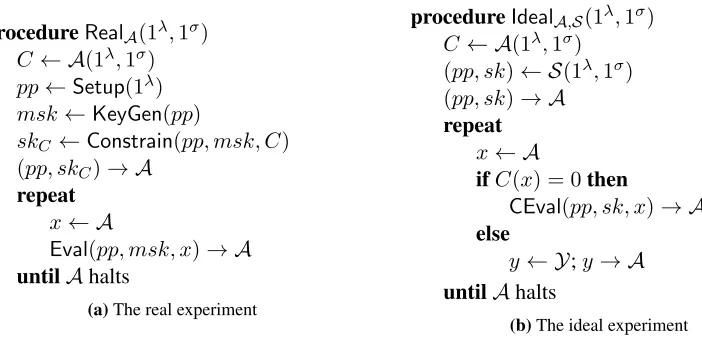
The above simulation-based definition simultaneously captures privacy of the constraining function, pseudorandomness on unauthorized inputs, and correctness of constrained evaluation on authorized inputs. The first two properties (privacy and pseudorandomness) follow because in the ideal experiment, the simulator must generate a constrained key without knowing the constraining function, and the adversary gets oracle access to a function that is uniformly random on unauthorized inputs.
For correctness, we claim that the real experiment is computationally indistinguishable from a modified one where each query x is answered as CEval(pp, skC, x) if x is authorized (i.e., C(x) = 0), and as Eval(pp, msk, x)otherwise. In particular, this implies thatEval(pp, msk, x) =CEval(pp, skC, x)with all
but negligible probability for all the adversary’s authorized queriesx. Indistinguishability of the real and modified experiments follows by a routine hybrid argument, with the ideal experiment as the intermediate one. In particular, the reduction that links the ideal and modified real experiments itself answers authorized queriesxusingCEval, and handles unauthorized queries by passing them to its oracle.
procedureRealA(1λ,1σ) C← A(1λ,1σ)
pp←Setup(1λ)
msk←KeyGen(pp)
skC ←Constrain(pp, msk, C)
(pp, skC)→ A repeat
x← A
Eval(pp, msk, x)→ A untilAhalts
(a)The real experiment
procedureIdealA,S(1λ,1σ) C← A(1λ,1σ)
(pp, sk)← S(1λ,1σ)
(pp, sk)→ A repeat
x← A
ifC(x) = 0then
CEval(pp, sk, x)→ A else
y← Y;y→ A untilAhalts
(b)The ideal experiment
Figure 2:The real and ideal experiments.
4.2 Construction
We now describe our construction of a CHC-PRF for domainX ={0,1}`and rangeY =Zmp , which handles
constraining circuits of sizeσ. It uses the following components:
• A pseudorandom functionPRF= (PRF.KG,PRF.Eval)having domain{0,1}`and rangeZmq , with
key space{0,1}κ.
• The shift hiding shiftable functionSHSF= (Setup,KeyGen,Eval,Shift,SEval,Sim)from Section 3, which has parametersq, Bthat appear in the analysis below.
For a boolean circuitCof size at mostσand somek∈ {0,1}κdefine the functionHC,k:{0,1}`→Zmq
as
HC,k(x) =C(x)·PRF.Eval(k, x) =
(
PRF.Eval(k, x) ifU(C, x) = 1
0 otherwise.
Notice that the size of (the binary decomposition of)HC,k is upper bounded by
wheresis the circuit size of (the binary decomposition of)PRF.Eval(k,·).
Construction 4.3. Our CHC-PRF with domainX ={0,1}`and rangeY =Zmp is defined as follows:
• Setup(1λ,1σ): outputpp←SHSF.Setup(1λ,1σ0)whereσ0 is defined as in Equation (4.1).
• KeyGen(pp): outputmsk←SHSF.KeyGen(pp).
• Eval(pp, msk, x∈ {0,1}`): computeyx =SHSF.Eval(pp, msk, x)and outputbyxep.
• Constrain(pp, msk, C): on input a circuitCof size at mostσ, sample a PRF keyk←PRF.KG(1λ)
and outputskC ←SHSF.Shift(pp, msk, HC,k).
• CEval(pp, skC, x): on input a constrained keyskCandx∈ {0,1}`, outputbSHSF.SEval(pp, skC, x)ep.
4.3 Security Proof
Theorem 4.4. Construction 4.3 is a constraint-hiding constrained PRF assuming the hardness ofLWEn−1,q,χ
and 1D-R-SIS(zσ0+τ+1)m,p,q,B(wherez, τ are respectively the lengths of fresh GSW ciphertexts and secret
keys as used inSHSF), the CPA security of the GSW encryption scheme, and thatPRFis a pseudorandom function.
Proof. Our simulatorS(1λ,1σ)for Construction 4.3 simply outputsSHSF.S(1λ,1σ0). Now letAbe any
polynomial-time adversary. To show thatSsatisfies Definition 4.2 we define a sequence of hybrid experiments and show that they are indistinguishable. Before defining the experiments in detail, we first define a particular “bad” event in all but one of them.
Definition 4.5. In each of the following hybrid experiments exceptH0, each queryxis answered asbyxep
for someyxthat is computed in a certain way. DefineBorderlineto be the event that at least one suchyxhas some coordinate inpq(Z+12) + [−B, B].
HybridH0: This is the ideal experimentIdealA,S.
HybridH1: This is the same as H0, except that on every unauthorized queryx (i.e., whereC(x) = 1), instead of returning a uniformly random value fromZmp , we chooseyx←Zmq and outputbyxep.
HybridH2: This is the same asH1, except that we abort the experiment ifBorderlinehappens.
HybridH3: This is the same asH2, except that we initially choose a PRF keyk←PRF.KG(1λ)and change how unauthorized queriesx(i.e., whereC(x) = 1) are handled, answering all queries according to a slightly modifiedCEval. Specifically, for any queryxwe answerbyxepwhere
yx=SHSF.SEval(pp, sk, x)−C(x)·PRF.Eval(k, x).
HybridH4: This is the same asH3, except that(pp, sk)are generated as in the real experiment. More formally we instantiatepp←SHSF.Setup(1λ,1σ0),msk←SHSF.KeyGen(pp)and computesk ← SHSF.Shift(pp, msk, HC,k).
HybridH5: This is the same asH4, except that we answer all evaluation queries as in theEvalalgorithm, i.e., we outputbyxepwhere
HybridH6: This is the same asH5, except that we no longer abort whenBorderlinehappens. Observe that this is exactly the real experimentRealA.
We now prove that adjacent pairs of hybrid experiments are indistinguishable.
Claim 4.6. ExperimentsH0andH1 are identical.
Proof. This follows directly from the fact thatpdividesq.
Claim 4.7. Assuming that 1D-R-SIS(zσ0+τ+1)m,p,q,B is hard, we haveH1 c
≈H2. In particular, inH1 the
eventBorderlinehappens with negligible probability.
Proof. LetAbe an adversary attempting to distinguish H1 andH2. We want to show that in H1 event
Borderline happens with negligible probability. Letx be a query made by A. If C(x) = 1 thenyx is uniformly random inZmq , so for anyi∈[m]we have
Pr[(yx)i∈ pq(Z+ 12) + [−B, B]]≤2·B·p/q= negl(λ).
IfC(x) = 0, the claim follows immediately by the border-avoiding property ofSHSF(Lemma 3.7).
Claim 4.8. IfPRFis a pseudorandom function thenH2
c
≈H3.
Proof. We use any adversaryAthat attempts to distinguishH2 fromH3 to build an adversaryA0 having the same advantage against the pseudorandomness ofPRF. HereA0 is given access to an oracleOwhich is eitherPRF.Eval(k,·)fork←PRF.KG(1λ), or a uniformly random functionf:{0,1}`→
Zmq . We define
A0to proceed as inH2to simulate the view ofA, except that on each queryxit sets
yx =SHSF.SEval(pp, sk, x)−C(x)· O(x)
and answersbyxep. Finally,A0outputs whateverAoutputs. Clearly, ifOisPRF.Eval(k,·)then the view
ofAis identical toH3, whereas if the oracle isf(·)then the view ofAis identical to its view inH2. This proves the claim.
Claim 4.9. Assuming the hardness ofLWEn−1,q,χand CPA-security ofGSW,H3
c
≈H4.
Proof. This follows immediately from the shift hiding property ofSHSF, i.e., Lemma 3.2.
Claim 4.10. H4 andH5are identical.
Proof. This follows by Corollary 3.9 and noticing that both experiments abort ifBorderlinehappens.
Claim 4.11. Under the hypotheses of Theorem 4.4, we haveH5
c
≈H6.
Proof. This follows by combining all the previous claims and recalling that we have proved thatBorderline
happens with negligible probability inH1.
5
Privately Programmable PRF
In this section we formally define privately programmable PRFs (PP-PRFs) and give a construction based on our shiftable PRF from Section 3.
5.1 Definitions
We start by giving a variety of definitions related to “programmable functions” and privately programmable PRFs. In particular, we give a simulation-based definition that is adapted from [BLW17].
Definition 5.1. A programmable function is a tuple (Setup,KeyGen,Eval,Program,PEval) of efficient algorithms having the following interfaces (where the domainX and rangeYmay depend on the security parameter):
• Setup(1λ,1k), given the security parameterλand a numberkof programmable inputs, outputs public
parameterspp.
• KeyGen(pp), given the public parameterspp, outputs a master secret keymsk.
• Eval(pp, msk, x), given the master secret key and an inputx∈ X, outputs somey∈ Y.
• Program(pp, msk,P ={(xi, yi)}), given the master secret keymskandkpairs(xi, yi)∈ X × Yfor
distinctxi, outputs a programmed keyskP.
• PEval(pp, skP, x), given a programmed keyskP and an inputx∈ X, outputs somey∈ Y.
We now give several definitions that capture various functionality and security properties for pro-grammable functions. We start with the following correctness property forprogrammedinputs.
Definition 5.2. A programmable function isstatistically programmableif for allλ, k = poly(λ)∈N, all
sets ofkpairsP ={(xi, yi)} ⊆ X × Y(with distinctxi), and alli∈[k]we have
Pr
pp←Setup(1λ,1k) msk←KeyGen(pp)
skP←Program(pp,msk,P)
[PEval(pp, skP, xi)6=yi] = negl(λ).
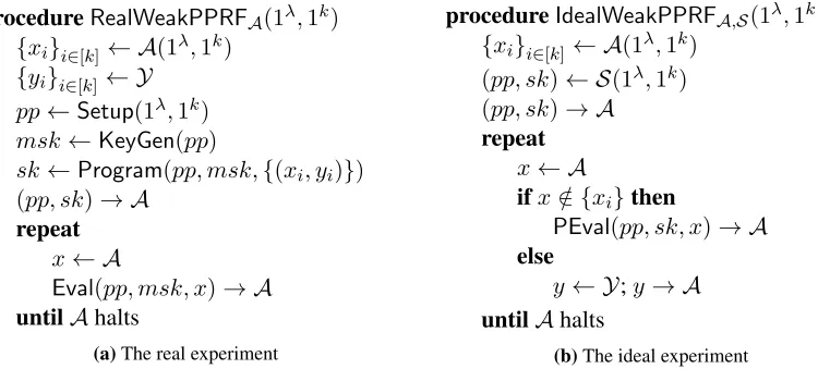
We now define a notion ofweaksimulation security, in which the adversary names the inputs at which the function is programmed, but the outputs are chosen at random (and not revealed to the adversary). As before, we always assume without loss of generality that the adversary never queries the same inputxmore than once in the various experiments we define.
Definition 5.3. A programmable function isweakly simulation secureif there is a PPT simulatorSsuch that for any PPT adversaryAand any polynomialk=k(λ),
{RealWeakPPRFA(1λ,1k)}λ∈N
c
≈ {IdealWeakPPRFA,S(1λ,1k)}λ∈N,
where RealWeakPPRFandIdealWeakPPRF are the respective views ofA in the procedures defined in Figure 3.
Similarly to Definition 4.2, the above definition simultaneously captures privacy of the programmed inputs given the programmed key, pseudorandomness on those inputs, and correctness ofPEvalonnon-programmed
procedureRealWeakPPRFA(1λ,1k) {xi}i∈[k]← A(1λ,1k)
{yi}i∈[k]← Y
pp←Setup(1λ,1k)
msk←KeyGen(pp)
sk←Program(pp, msk,{(xi, yi)})
(pp, sk)→ A repeat
x← A
Eval(pp, msk, x)→ A untilAhalts
(a)The real experiment
procedureIdealWeakPPRFA,S(1λ,1k) {xi}i∈[k]← A(1λ,1k)
(pp, sk)← S(1λ,1k)
(pp, sk)→ A repeat
x← A
ifx /∈ {xi}then
PEval(pp, sk, x)→ A else
y← Y;y→ A untilAhalts
(b)The ideal experiment
Figure 3:The (weak) real and ideal experiments.
Definition 5.4. A programmable function is aweak privately programmable PRFif it is statistically pro-grammable (Definition 5.2) and weakly simulation secure (Definition 5.3).
We now define a notion of (non-weak) simulation security for programmable functions. This differs from the weak notion in that the adversary specifies the programmed inputsandcorresponding outputs, and the simulator in the ideal game is also given these input-output pairs. The simulator needs this information because otherwise the adversary could trivially distinguish the real and ideal experiments by checking whether
PEval(pp, skP, xi) = yi for one of the programmed input-output pairs(xi, yi). Simulation security itself
therefore does not guarantee any privacy of the programmed inputs; below we give a separate simulation-based definition which does.
procedureRealPPRFA(1λ,1k) P ={(xi, yi)} ← A(1λ,1k)
pp←Setup(1λ,1k)
msk←KeyGen(pp)
skP ←Program(pp, msk,P) (pp, skP)→ A
repeat
x← A
Eval(pp, msk, x)→ A untilAhalts
(a)The real experiment
procedureIdealPPRFA,S(1λ,1k) P ={(xi, yi)} ← A(1λ,1k)
(pp, skP)← S(1λ,P) (pp, skP)→ A
repeat
x← A
ifx /∈ {xi}then
PEval(pp, skP, x)→ A
else
y← Y;y→ A untilAhalt
(b)The ideal experiment
Figure 4:The real and ideal experiments
Definition 5.5. A programmable function issimulation secureif there is a PPT simulatorSsuch that for any PPT adversaryAand any polynomialk=k(λ),
{RealPPRFA(1λ,1k)}λ∈N
c
whereRealandIdealare the respective views ofAin the procedures defined in Figure 4.
We mention that a straightforward hybrid argument similar to one from [BKM17] shows that simulation security implies that(KeyGen,Eval)is a pseudorandom function.
Finally, we define a notion of privacy for the programmed inputs. This says that a key programmed on adversarially chosen inputs andrandomcorresponding outputs (that are not revealed to the adversary) does not reveal anything about the programmed inputs.
procedureRealPPRFPrivacyA(1λ,1k) {xi}i∈[k]← A(1λ,1k)
{yi}i∈[k]← Y
pp←Setup(1λ,1k)
msk←KeyGen(pp)
sk←Program(pp, msk,{(xi, yi)})
(pp, sk)→ A
(a)The real experiment
procedureIdealPPRFPrivacyA,S(1λ,1k) {xi}i∈[k]← A(1λ,1k)
(pp, sk)← S(1λ,1k)
(pp, sk)→ A
(b)The ideal experiment
Figure 5:The real and ideal privacy experiments
Definition 5.6. A programmable function isprivately programmableif there is a PPT simulatorSsuch that for any PPT adversaryAand any polynomialk=k(λ),
{RealPPRFPrivacyA(1λ,1k)}λ∈N c
≈ {IdealPPRFPrivacyA(1λ,1k)}λ∈N,
whereRealPPRFPrivacyandIdealPPRFPrivacyare the respective views ofAin the procedures defined in Figure 5.
We now give our main security definition for PP-PRFs.
Definition 5.7. A programmable function is aprivately programmable PRFif it is statistically programmable, simulation secure, and privately programmable.
5.2 From Weak PP-PRFs to PP-PRFs
In this section we describe a general construction of a privately programmable PRF from any weak privately programmable PRF. LetΠ0 = (Setup,KeyGen,Eval,Program,PEval) be a programmable function with domain X and range Y, where we assume that Y is a finite additive group. The basic idea behind the construction is simple: define the function as the sum of two parallel copies of Π0, and program it by programming the copies according to additive secret-sharings of the desired outputs. Each component is therefore programmed to uniformly random outputs, as required by weak simulation security.
Construction 5.8. We construct a programmable functionΠas follows:
• Π.Setup(1λ,1k): generatepp
i←Π0.Setup(1λ,1k)fori= 1,2and outputpp= (pp1, pp2).
• Π.KeyGen(pp): on inputpp= (pp1, pp2)generatemski ←Π0.KeyGen(ppi)fori= 1,2, and output
• Π.Eval(pp, msk, x): on inputpp= (pp1, pp2),msk= (msk1, msk2), andx∈ X output
Π0.Eval(pp1, msk1, x) + Π0.Eval(pp2, msk2, x).
• Π.Program(pp, msk,P): on inputpp= (pp1, pp2),msk= (msk1, msk2),kpairs(xi, yi)⊂ X × Y,
first sample uniformly randomri ← Yfori∈[k], then outputskP = (sk1, sk2)where
sk1 ←Π0.Program(pp1, msk1,P1 ={(xi, ri)})
sk2 ←Π0.Program(pp2, msk2,P2 ={(xi, yi−ri)}).
• Π.PEval(pp, skP, x): on inputpp= (pp1, pp2),skP = (sk1, sk2), andx∈ X output
Π0.PEval(pp1, sk1, x) + Π0.PEval(pp2, sk2, x).
Theorem 5.9. If Π0 is a weak privately programmable PRF then Construction 5.8 is a privately pro-grammable PRF.
Proof. This follows directly from Theorem 5.10 and Theorem 5.15, which respectively prove the simulation security and private programmability of Construction 5.8, and from the statistical programmability ofΠ0, which obviously implies the statistical programmability of Construction 5.8.
Theorem 5.10. IfΠ0is a weak privately programmable PRF thenΠis simulation secure.
Proof. Let S0 be the simulator algorithm for the weak simulation security of Π0 (Definition 5.3). Our simulatorS(1λ,P ={(x
i, yi)})for the simulation security ofΠ(Definition 5.5) works as follows:
1. Compute(pp2, sk2)← S0(1λ,1k)wherek=|P|.
2. Computepp1 ←Π0.Setup(1λ,1k),msk1 ←Π0.KeyGen(pp1), and
sk1 ←Π0.Program(pp1, msk1,{(xi, yi−Π0.PEval(pp2, sk2, xi))}).
3. Output(pp= (pp1, pp2), sk = (sk1, sk2)).
We now define the following hybrids and show that they are indistinguishable.
HybridH0: This is the real experiment RealPPRFA from Figure 4, up to negligible statistical distance. Specifically: the adversaryAfirst outputs{(xi, yi)}. We then generateppi ←Π0.Setup(1λ,1k)and
mski ←Π0.KeyGen(ppi)fori= 1,2. We choose uniformly randomri← Y fori∈[k], and let
sk1 ←Π0.Program(pp1, msk1,{(xi, ri)})
sk2 ←Π0.Program(pp2, msk2,{(xi, yi−Π0.PEval(pp1, sk1, xi))}).
(Note that inyi−riwe have replacedri with a call toΠ0.PEval; these are equivalent up to negligible
HybridH1: This is the same as the previous experiment, except we change howpp1andsk1are generated, and how queries are answered. We generate(pp1, sk1)← S0(1λ,1k), and no longer generatemsk1. To answer each queryx, ifx /∈ {xi}then we outputΠ0.PEval(pp1, sk1, x) + Π0.Eval(pp2, msk2, x); otherwise, we output a uniformly random value fromY.
HybridH2: This is the same as the (real) experimentH0, except that for queriesx /∈ {xi}, just as inH1we outputΠ0.PEval(pp1, sk1, x) + Π0.Eval(pp2, msk2, x).
HybridH3: This is the same as the previous experiment, except we replaceyi−Π0.PEval(pp1, sk1, xi)
withyi−ri, then we swap the roles ofriandyi−ri(usingriwhen computingsk2andyi−riwhen
computingsk1), then replaceyi−riwithyi−Π0.PEval(pp2, sk2, xi).
HybridH4: This is the same as the previous experiment, except we change howpp2andsk2are generated and how queries are answered. We generate(pp2, sk2)← S0(1λ,1k), and no longer generatemsk2. To answer a queryx, ifx /∈ {xi}then we respond withΠ0.PEval(pp1, sk1, x) + Π0.PEval(pp2, sk2, x); otherwise, we respond with a uniformly random value fromY.
Observe that this hybrid is identical to the ideal experimentIdealPPRFA,S0 from Figure 4.
We now show that adjacent hybrid experiments are indistinguishable.
Claim 5.11. We haveH0
c
≈H1.
Proof. LetAbe an adversary attempting to distinguishH0fromH1. We build an adversaryA0against the weak simulation security ofΠ0that runsAinternally and works as follows:
• WhenAoutputs{(xi, yi)},A0outputs{xi}and receives some(pp1, sk1).
• A0computespp2←Π0.Setup(1λ,1k),msk2 ←Π0.KeyGen(pp2), and
sk2 ←Π0.Program(pp2, msk2,{(xi, yi−Π0.PEval(pp1, sk1, xi))}),
and gives(pp= (pp1, pp2), sk = (sk1, sk2))toA.
• WhenAqueries somex,A0queriesxand receives a responsey0, and returnsy0+Π0.Eval(pp2, msk2, x) as the answer toA.
Because theriare uniformly random inH0, it is straightforward to verify that ifA0is in theRealWeakPPRF (respectively,IdealWeakPRF) experiment, then the view ofAis identical to its view inH0(resp.,H1). So by weak simulation security ofΠ0, we haveH0
c
≈H1.
Claim 5.12. We haveH1
c
≈H2.
Proof. LetAbe an adversary attempting to distinguishH1fromH2. We build an adversaryA0against the weak simulation security ofΠ0 that works exactly like theA0from the proof of Claim 5.11, except for how it handles queriesx: if x /∈ {xi}, thenA0 responds withΠ0.PEval(pp1, sk1, x) + Π0.Eval(pp2, msk2, x); otherwise,A0queriesxand receives a responsey0, then responds withy0+ Π0.Eval(pp2, msk2, x).
It is straightforward to verify that ifA0is in experimentIdealWeakPPRF(respectively,IdealRealPPRF), then the view ofAis identical to its view inH1(resp.,H2). So by weak simulation security ofΠ0, we have H0
c
Claim 5.13. We haveH2
s
≈H3.
Proof. This follows by statistical programmability, the fact thatri, yi−riis a random secret sharing ofyi,
so we can swap their roles, and statistical programmability again.
Claim 5.14. We haveH3
c
≈H4.
Proof. This is entirely symmetrical to the proof of Claim 5.11, so we omit a detailed proof.
This completes the proof of Theorem 5.10.
Theorem 5.15. IfΠ0is weakly simulation secure thenΠis privately programmable.
Proof. LetS0 be the simulator algorithm for the weak simulation security ofΠ0. Our simulatorS(1λ,1k)
for the private programmability ofΠ simply generates(ppi, ski) ← S0(1λ,1k) fori = 1,2 and outputs
(pp= (pp1, pp2), sk= (sk1, sk2)). To show thatSsatisfies Definition 5.7 we define the following hybrids and show that they are indistinguishable.
HybridH0: This is the experimentRealPPRFPrivacyAfrom Figure 5.
HybridH1: This experiment is the same as the previous one, except that we generate (pp1, sk1) ← S0(1λ,1k).
HybridH2: This experiment is the same as the previous one, except that we generate (pp2, sk2) ← S0(1λ,1k). Observe that this experiment is identical to the experiment IdealPPRFPrivacyA,S from Figure 5.
Claim 5.16. We haveH0
c
≈H1.
Proof. LetAbe an adversary attempting to distinguishH0andH1. We build an adversaryA0against the weak simulation security ofΠ0, which runsAinternally. WhenAoutputs{xi},A0also outputs{xi}, receiving
(pp1, sk1)in response. ThenA0 generatespp2 ← Π0.Setup(1λ,1k)and msk2 ← Π0.KeyGen(pp2), and chooses uniformly randomri ← Yfori∈[k]. It then generatessk2←Π0.Program(pp2, msk2,{(xi, ri)}).
Finally it gives (pp = (pp1, pp2), sk = (sk1, sk2)) to A. It is straightforward to see that if A0 is in
RealWeakPPRF(respectively,IdealWeakPPRF) then the view ofAis identical to its viewH0(resp.,H1). So by weak simulation security ofΠ0, we haveH0
c
≈H1.
Claim 5.17. We haveH1
c
≈H2.
Proof. This is entirely symmetrical to the proof of Claim 5.16, so we omit it.
5.3 Construction of Weak Privately Programmable PRFs
In this section we construct a weak privately programmable PRF from our shiftable function of Section 3. We first define the auxiliary function that the construction will use. For{(xi,yi)}i∈[k]⊂ {0,1}
`×
Zmq where
thexi are distinct, define the functionH{(xi,wi)}i∈[k]:{0,1}
`→
Zmq as
H{(xi,wi)}i∈[k](x)
(
wi ifx=xi for somei,
0 otherwise.
Notice that the circuit size ofH{(xi,wi)}i∈[k] is upper bounded by someσ
0 = poly(n, k,logq).
Construction 5.18. Our weak privately programmable PRF with input spaceX ={0,1}`and output space
Y =Zmp uses the SHSF from Section 3 with parametersq, B chosen as in Section 3.4, and is defined as
follows:
• Setup(1λ,1k): Outputpp←SHSF.Setup(1λ,1σ0).
• KeyGen(pp): Outputmsk←SHSF.KeyGen(pp).
• Eval(pp, msk, x∈ {0,1}`): Computeyx=SHSF.Eval(pp, msk, x)and outputbyxep.
• Program(pp, msk,P): Given kpairs (xi,yi) ∈ {0,1}`×Zmp where thexi are distinct, for each
i∈[k]computewi as follows: chooseyi0 ←Zmq uniformly at random conditioned onby0iep =yi, and
set
wi =y0i−SHSF.Eval(pp, msk, xi).
OutputskP ←SHSF.Shift(pp, msk, H{(xi,wi)}).
• PEval(pp, skP, x): outputbSHSF.SEval(pp, skP, x)ep.
5.4 Security Proof
Theorem 5.19. Construction 5.18 is a weak privately programmable PRF (Definition 5.4) assuming the hardness ofLWEn−1,q,χand 1D-R-SIS(zσ0+τ+1)m,p,q,B (wherez, τ are respectively the lengths of fresh GSW
ciphertexts and secret keys as used inSHSF) and the CPA security of the GSW encryption scheme.
Proof. The proof follows immediately by Theorem 5.20 and Theorem 5.28 below.
Theorem 5.20. Assuming the hardness ofLWEn−1,q,χand 1D-R-SIS(zσ0+τ+1)m,p,q,B and the CPA security
of the GSW encryption scheme, Construction 5.18 is weakly simulation secure.
Proof. Our simulatorS(1λ,1k)for Construction 5.18 simply outputs(pp, sk)←SHSF.S(1λ,1σ0). LetA
be any polynomial-time adversary. To show thatSsatisfies Definition 5.5 we define a sequence of hybrid experiments and show that they are indistinguishable.
HybridH0: This is the simulated experimentIdealWeakPPRFA,S (Figure 3).
HybridH1: This is the same as the previous experiment, except that on queryx∈ {xi}, instead of returning
HybridH2: This is the same as the previous experiment, except that we abort if the event Borderline happens, whereBorderlineis as in Definition 4.5.
HybridH3: This is the same as the previous experiment, except that we initially choose uniformly random
w0i ← Zm
q for i ∈ [k]and change how queries for x ∈ {xi} are answered (the “else” clause in IdealWeakPPRFA,S): forx=xj, we answer asbyxep, where
yx =SHSF.SEval(pp, sk, x)−wj0.
HybridH4: This is the same as the previous experiment, except that we generateppandskas follows: we generatepp←Setup(1λ,1k),msk←KeyGen(pp)andsk ←SHSF.Shift(pp, msk, H
{(xi,w0i)}). HybridH5: This is the same as the previous experiment, except that we answer all queries as in theEval
algorithm, i.e., we output
bSHSF.Eval(pp, msk, x)ep.
HybridH6: This is the same as the previous experiment, except that here we generateskas in the real game. Specifically, for eachi∈[k]we choose a uniformly random vectoryi ←Zmp and uniformly random yi0 ←Zmq conditioned onby0iep =yi, and then set
wi=yi0−SHSF.Eval(pp, msk, x).
We then setsk←SHSF.Shift(pp, msk, H{(xi,wi)}).
HybridH7: This is the same as the previous experiment, except that we no longer abort whenBorderline happens. Observe that this is the real experimentIdealRealPPRFA(Figure 3).
Claim 5.21. ExperimentsH0andH1are identical.
Proof. This follows directly from the fact thatpdividesq.
Claim 5.22. Under 1D-R-SIS(zσ0+τ+1)m,p,q,B assumption, H1 c
≈ H2. In particular, in H1 the event
Borderlinehappens with negligible probability.
Proof. The proof is identical to the one for Claim 4.7.
Claim 5.23. ExperimentsH2andH3are identical.
Proof. This simply follows by observing that forx ∈ {xi},yxis distributed uniformly at random in both
hybridsH2andH3.
Claim 5.24. Assuming the hardness ofLWEn−1,q,χand CPA-security ofGSW,H3
c
≈H4.
Proof. This follows immediately from the shift-hiding property ofSHSF(Lemma 3.2).
Claim 5.25. H4 andH5are identical.
Claim 5.26. ExperimentsH5andH6are identical.
Proof. Becausepdividesq, for eachi∈[k]eachy0iinH6is uniformly distributed, which implies that each
wiis also uniformly distributed, as inH5.
Claim 5.27. Assuming the hypotheses of Theorem 5.20,H6
c
≈H7.
Proof. This follows by combining all the previous claims and recalling thatBorderlinehappens with negligi-ble probability inH1.
This completes the proof of Theorem 5.20.
Theorem 5.28. Construction 5.18 is statistically programmable.
Proof. Fix anyP ={(xi,yi)}i∈[k]⊂ X × Y. We need to show that for anyi∈[k],
Pr
pp←Setup(1λ,1k) msk←KeyGen(pp)
skP←Program(pp,msk,P)
j
SHSF.SEval(pp, skP, xi)
m
p 6=yi
= negl(λ). (5.1)
By Lemma 3.8 we have
SHSF.SEval(pp, skP, xi)≈SHSF.Eval(pp, msk, xi) +H{(xi,wi)}(xi)
=SHSF.Eval(pp, msk, xi) +wi
=y0i,
where the approximation hides some B-bounded error and the last equality holds because wi = yi0 − SHSF.Eval(pp, msk, xi). Becauseyi0 is chosen uniformly at random such thatby0iep =yi, the probability
that some coordinate ofSHSF.SEval(pp, skP, xi)is in qp(Z+12) + [−B, B]is at most2mBp/q= negl(λ),
which establishes Equation (5.1).
References
[Ajt96] M. Ajtai. Generating hard instances of lattice problems. Quaderni di Matematica, 13:1–32, 2004. Preliminary version in STOC 1996.
[BGG+14] D. Boneh, C. Gentry, S. Gorbunov, S. Halevi, V. Nikolaenko, G. Segev, V. Vaikuntanathan, and D. Vinayagamurthy. Fully key-homomorphic encryption, arithmetic circuit ABE and compact garbled circuits. InEUROCRYPT, pages 533–556. 2014.
[BGI+01] B. Barak, O. Goldreich, R. Impagliazzo, S. Rudich, A. Sahai, S. P. Vadhan, and K. Yang. On the (im)possibility of obfuscating programs. J. ACM, 59(2):6:1–6:48, 2012. Preliminary version in CRYPTO 2001.
[BGI14] E. Boyle, S. Goldwasser, and I. Ivan. Functional signatures and pseudorandom functions. In
[BGI15] E. Boyle, N. Gilboa, and Y. Ishai. Function secret sharing. InEUROCRYPT, pages 337–367. 2015.
[BKM17] D. Boneh, S. Kim, and H. W. Montgomery. Private puncturable PRFs from standard lattice assumptions. InEUROCRYPT, pages 415–445. 2017.
[BLMR13] D. Boneh, K. Lewi, H. W. Montgomery, and A. Raghunathan. Key homomorphic PRFs and their applications. InCRYPTO, pages 410–428. 2013.
[BLP+13] Z. Brakerski, A. Langlois, C. Peikert, O. Regev, and D. Stehl´e. Classical hardness of learning with errors. InSTOC, pages 575–584. 2013.
[BLW17] D. Boneh, K. Lewi, and D. J. Wu. Constraining pseudorandom functions privately. InPKC, pages 494–524. 2017.
[BP14] A. Banerjee and C. Peikert. New and improved key-homomorphic pseudorandom functions. In
CRYPTO, pages 353–370. 2014.
[BPR12] A. Banerjee, C. Peikert, and A. Rosen. Pseudorandom functions and lattices. InEUROCRYPT, pages 719–737. 2012.
[BTVW17] Z. Brakerski, R. Tsabary, V. Vaikuntanathan, and H. Wee. Private constrained PRFs (and more) from LWE. InTCC, pages ??–?? 2017.
[BV15] Z. Brakerski and V. Vaikuntanathan. Constrained key-homomorphic PRFs from standard lattice assumptions - or: How to secretly embed a circuit in your PRF. InTCC, pages 1–30. 2015.
[BW13] D. Boneh and B. Waters. Constrained pseudorandom functions and their applications. In
ASIACRYPT, pages 280–300. 2013.
[CC17] R. Canetti and Y. Chen. Constraint-hiding constrained PRFs for nc1 from LWE. InEUROCRYPT, pages 446–476. 2017.
[CHN+16] A. Cohen, J. Holmgren, R. Nishimaki, V. Vaikuntanathan, and D. Wichs. Watermarking cryptographic capabilities. InSTOC, pages 1115–1127. 2016.
[GGH+13] S. Garg, C. Gentry, S. Halevi, M. Raykova, A. Sahai, and B. Waters. Candidate indistin-guishability obfuscation and functional encryption for all circuits. In FOCS, pages 40–49. 2013.
[GGM84] O. Goldreich, S. Goldwasser, and S. Micali. How to construct random functions. J. ACM, 33(4):792–807, 1986. Preliminary version in FOCS 1984.
[GSW13] C. Gentry, A. Sahai, and B. Waters. Homomorphic encryption from learning with errors: Conceptually-simpler, asymptotically-faster, attribute-based. InCRYPTO, pages 75–92. 2013.
[GVW15a] S. Gorbunov, V. Vaikuntanathan, and H. Wee. Predicate encryption for circuits from LWE. In
CRYPTO, pages 503–523. 2015.
[KPTZ13] A. Kiayias, S. Papadopoulos, N. Triandopoulos, and T. Zacharias. Delegatable pseudorandom functions and applications. InCCS, pages 669–684. 2013.
[KW17] S. Kim and D. J. Wu. Watermarking cryptographic functionalities from standard lattice assump-tions. InCRYPTO, pages 503–536. 2017.
[MP12] D. Micciancio and C. Peikert. Trapdoors for lattices: Simpler, tighter, faster, smaller. In
EUROCRYPT, pages 700–718. 2012.
[MR04] D. Micciancio and O. Regev. Worst-case to average-case reductions based on Gaussian measures.
SIAM J. Comput., 37(1):267–302, 2007. Preliminary version in FOCS 2004.
[Pei09] C. Peikert. Public-key cryptosystems from the worst-case shortest vector problem. InSTOC, pages 333–342. 2009.
[PRS17] C. Peikert, O. Regev, and N. Stephens-Davidowitz. Pseudorandomness of Ring-LWE for any ring and modulus. InSTOC, pages 461–473. 2017.