Copyright by
Muneeza Azmat 2018
The Report Committee for Muneeza Azmat Certifies that this is the approved version of the following Report:
Multi-class Segmentation of Brain Tumor using
Convolution Neural Network
APPROVED BY
SUPERVISING COMMITTEE:
George Biros, Supervisor Thomas Yankeelov
Multi-class Segmentation of Brain Tumor using
Convolution Neural Network
by
Muneeza Azmat
REPORT
Presented to the Faculty of the Graduate School of The University of Texas at Austin
in Partial Fulfillment of the Requirements
for the Degree of
Master of Science in Computational Science, Engineering, and Mathematics
THE UNIVERSITY OF TEXAS AT AUSTIN May 2018
Multi-class Segmentation of Brain Tumor using
Convolution Neural Network
Muneeza Azmat, M.S.C.S.E.M The University of Texas at Austin, 2018
Supervisor: George Biros
In this report a fully Convolution Neural Network (CNN) architecture is used to segment multi-modal Brain Tumors from Magnetic Resonance (MR) images. Due to the challenges in manual segmentation, computerized brain tu-mor segmentation is one of the most important challenges in medical imaging. The fully convolutional structure of the network makes it faster than any net-work with a dense fully connected layer. The two phase training and entropy sampling of data makes it easier to learn tumor boundaries and overcome the data imbalance problem.
Table of Contents
Abstract v
List of Tables vii
List of Figures viii
Chapter 1. 1 1.1 Introduction . . . 1 1.2 Mathematical Formulation . . . 3 1.2.1 Convolution . . . 4 1.2.2 Activation Function . . . 4 1.2.3 Loss function . . . 6 1.2.4 Regularization . . . 7 1.2.5 Optimization . . . 8 1.3 Network . . . 11 Chapter 2. 12 2.1 Implementation Details . . . 12 2.1.1 Pre-processing . . . 12 2.1.2 Patch Extraction . . . 13
2.1.3 Hyper-parameter selection and tuning . . . 14
2.1.4 Training . . . 17
2.2 Results . . . 18
2.3 Conclusion . . . 19
List of Tables
List of Figures
1.1 Architecture of the Convolution Neural Network . . . 11 2.1 High entropy filter results with different neighborhood sizes . . 13 2.2 Sampled values from uniform grid G (a) Coarse Grid (b) Fine
Grid . . . 15 2.3 Tuning (α,β) (a) Coarse grid (b) Fine grid. . . 16 2.4 Tuning (λ1,λ2) (a) Training loss (b) Validation loss . . . 16
2.5 (a) Training results for different adaptive methods. (b) Valida-tion accuracy of each method. (c) Learning rate decay schedule. (d) Momentum increase schedule . . . 17 2.6 Training results for Phase-1 (top) and Phase-2 (bottom) for
different epochs . . . 18 2.7 Validation results for Phase-1 (top) and Phase-2 (bottom) for
Chapter 1
1.1
Introduction
Despite having been studied for centuries cancer remains one of the biggest challenges in modern medicine. Malignant brain tumors are one of the most lethal cancers, among these, Gliomas are the most commonly occurring brain malignancies. They are usually classified into sub-regions based on their histological heterogeneity i.e. edema, necrotic core, enhancing and nonenhanc-ing tumor core.
To contain the damage caused by tumors, recover neurological functions, and consequently increase the survival rate, early diagnosis of the tumor is essen-tial. Magnetic resonance imaging (MRI) is the diagnostic tool of choice, it provides detailed images of the brain and has multiple modes to better distin-guish between healthy and tumorous tissues, e.g. T1 (spin-lattice relaxation), T1-contrasted (T1C), T2 (spin-spin relaxation) and fluid attenuation inversion recovery (FLAIR) pulse sequence.
In clinical practice brain tumors are identified and segmented manually from MRI images. This is a tedious and time-consuming process and is becoming increasingly complex with advancement in MRI imaging. This manual analysis is also prone to errors due to inter-operator variability. All these problems
de-mand computerized methods for medical image analysis, e.g. automatic brain tumor identification, segmentation, and visualization to assist physicians in qualitative diagnosis.
Automatic segmentation of brain tumors is a very challenging problem, Gliomas are typically non-local with diffused and irregular boundaries. They also vary greatly in their shape, size, and location in the brain. Data obtained from dif-ferent machines is also prone to variation and biases. The use of multiple MRI modalities for effective segmentation also adds complexity to the problem. In addition to this it is a highly data imbalance problem with more than 98% of the brain comprising of healthy tissues and the tumor core making up less than 1% of the brain.
Automatic brain tumor segmentation methods are based on models that can roughly be divided into discriminative and generative models [5].
Generative models rely heavily on prior knowledge of the location, appearance and spatial extent of tumorous and healthy tissues. They typically work by using an atlas computed from healthy brains as priors. This along with the test brain is then used to compute posterior probabilities of healthy tissues on the test brain.
Discriminative models on the other hand directly learn the relationship be-tween input and segmentation label by extracting useful linear and non-linear features from the image data. They typically work by extracting features like local intensity difference [2], Gabor filterbanks [7], gradients, symmetry anal-ysis etc. Standard classification algorithms e.g., Support Vector Machines or
decision trees are then used to classify these features. The learned classifica-tion maps are then applied to new data for segmentaclassifica-tion. Even though these methods dont rely on prior knowledge of brains anatomy they typically require large amounts of data for training the classifiers.
Recently discriminative models using deep Convolution Neural Networks (CNN) have shown a lot of promise, in fact most state of the art methods currently employ CNNs [8]. The fully convolutional architecture of these methods makes them faster than their generative counterparts. Havaei et al. [4] presented mul-tiple fully convolutional architectures for segmentation of brain tumors using neural networks of varying complexity.
The work in this report is based on the work of Havaei et al [4], with several modifications in the formulation and sampling implemented with a different software infrastructure.
First a mathematical description of the network and its components is given. then the implementation is detailed in the second chapter describing in detail the data sampling, hyper-parameter tuning and training techniques. Finally the results are shown followed by a discussion
1.2
Mathematical Formulation
The network is based on the Deep Convolution neural network (CNN) proposed by [4] which is a two layer patch-wise CNN. The input is a multi-modal MRI from the BRATS data set. This 3D image has four channels:
T1,T2,FLAIR, and T1ce. The segmentation is performed per axial slice, thus the model processes 2D multi-modal slices. To perform classification multiple patches of size n x n are extracted from each axial slice and the network is trained to classify the center pixel of each patch.
1.2.1 Convolution
The building blocks of this network are convolution layers, these layers generate feature maps for a given input, the features extracted depend on the parameters of the convolution filter. The values of these parameters are learned during training. Given an input X and a convolution filter (kernel)
Wof dimensions w1×w2, the convolution operation is given by:
(X∗W)ij = w1−1 X m=0 w2−1 X n=0 X(i−m, j−n)W(m, n) (1.1) The size of a convolution filter is also called itsReceptivef ield. For an input withC input channels (or modalities) the feature map Fis computed as:
F =b+ C
X
m=1
(Xm∗Wm) (1.2)
whereWm is the convolution kernel formth input Xm and b is a bias term.
1.2.2 Activation Function
Some important features of the image might not be linearly dependent on the input, to extract such features a non-linear activation function is applied
element-wise
e
F =g(b+X m
(Xm∗Wm)) (1.3)
whereg is the activation function. The non-linear activation functions used in this network are discusses below.
Maxout: Proposed in [3] the Maxout non-linearity is shown to be effective at extracting useful features especially when used with dropout reg-ularization (discussed later). The function takes multiple feature maps (FMs) as its input and takes the element-wise maximum over them. The kth FM resulting from maxout on s convolution FMs{Fk+1, ..., Fk+s} of size m×n is simply:
e
Fk,i,jmax =max{Fk+1,i,j, .., Fk+s,i,j} where i= 1, .., m and j = 1, .., n (1.4) Max pooling: Max-pooling keeps the maximum value in a moving window of size p×p over the feature map, the amount by which the filter shifts (horizonally and vertically) is called stride. This operation shrinks the size of the feature map and introduces local translation invariance. The output of a max pooling layer applied toFemax with stride= 1 can be written as:
e
Fk,i,jpool = max{Fk,m,n:i≤m≤i+p−1, j ≤n ≤j+p−1} (1.5) Softmax: Softmax is used in the final layer of the neural network, it normalizes the values of a vector such that they add up to 1 i.e. giving a
multinomial distribution. Let F be a k dimensional vector output of a fully connected layer, then the softmax output is given as:
σi(F) = eFi Pk i eFi and i= 1, .., k (1.6) 1.2.3 Loss function
The output of the network can be interpreted as a multinomial distri-bution{qX(i)}i∈Labels where qX(i) is the probability that the evaluated input
Xbelongs to tumor classi. Softmax applied prior the output ensures that for each input X the output is indeed a probability distribution
X
i∈Labels
qX(i) = 1 (1.7)
One can construct another distribution pX(i) corresponding to the Ground
Truth (GT) segmentation for each X.The loss function is then defined as the mismatch between the obtained and desired probability distributions, which is given by the Kullback-Leibler divergence (KL-Divergence) of the two distri-butions. For discrete distributions over i labels the divergence of q from p is defined as: L(X) = DKL(p||q) = − X i pX(i) ln qX(i) pX(i) (1.8) Note that the KL-Divergence is well defined because
qX(i) = σi(F(X))∈(0,1) and lim
L(X) =X i pX(i) lnpX(i)− X i pX(i) lnqX(i) (1.10) where H(pX) = X i pX(i) lnpX(i) (1.11) Is the Shannon Entropy of p for a given input X, since for all training data GT labels are already knownH(p) = 0
L(X) =− X
i∈Labels
pX(i) lnqX(i) (1.12)
1.2.4 Regularization
To reduce the generalization error following regularization techniques have been used in the network:
Max-norm: The absolute value of the weight is bounded in each layer of the network. This allows the network to have a bigger value of learning rate.
|W|< c (1.13)
This is implemented during training by clipping the gradient norm (see opti-mization) if it exceeds a certain value.
L1 and L2: The L1 and L2 norms of the weights are added as a penalty to the total loss function to prevent over-fitting. The total loss
func-tion after regularizafunc-tion looks like: L(X, W) = −X
i
pX(i) lnqX(i) +λ1||W||1+λ2||W||2 (1.14)
where λ1 and λ2 are regularization coefficients
Early stopping: A validation set is used to limit the training time i.e. the training is stopped when the performance on validation set stops improving.
Dropout: Dropout works by adding noise to the input (or hidden layers) of the network this reduces co-adaptations of inputs (or neurons) and effectively reduces the generalization error. all units of each layer are multiplied with Pd – the probability of retaining a unit.
As proposed in [3] the element-wise multiplication with Pd is performed right before convolution . In our network we apply dropout to the input units with Pd = 0.8 and Pd = 0.5 for hidden units as suggested in [6]
1.2.5 Optimization
The goal is to bring the learned distribution qX as close to the GT distribution pX by minimizing the loss function L(X). To perform this task Stochastic Gradient Descent (SGD) is used.
For a given inputX we can write L(X) as a function of the parameters (W, b) L(X) = −X i pX(i) lnqX(i) (1.15) L(X) = −X i pX(i) lnσi(F(X)) (1.16) LX(W, b) = − X i pX(i) lnσi(b+ X m (X∗W)) (1.17) LX(W, b, λ1, λ2) = − X i pX(i) lnσi(b+ X m (X∗W)) +λ1||W||1+λ2||W||2 (1.18) To minimize this loss we need to calculate the gradient
∇LX(W, b, λ1, λ2) = ∂L ∂W ∂L ∂b ∂L ∂λ1 ∂L ∂λ2 (1.19) where ∂LX ∂W =− X i pX(i) ∂ ∂W lnσi(b+ X m (X∗W)) (1.20) ∂LX ∂b =− X i pX(i) ∂ ∂blnσi(b+ X m (X∗W)) (1.21) ∂LX ∂λ1 =||W||1 (1.22) ∂LX ∂λ2 =||W||2 (1.23)
The first two terms are calculated by taking derivatives of the filters (kernels) and activation functions in each layer and then using chain rule.
To train the network the loss is minimized using stochastic gradient descent. In each iterationj of SGD the parameters are updated via the following recursive relation
Wj+1 =Wj −α∇LX(W, b, λ1, λ2)j (1.24)
Where αcalled theLearningRateis an important hyper-parameter and needs to be tuned prior to training (discussed in Chapter 2) . For a mini-batch of N samples the average is used
Wj+1 =Wj − α N N X X=1 ∇LX(W, b, λ1, λ2)j (1.25)
To improve optimization SGD is used with a momentum correction. This helps the optimizer escape local minima. For a learning rateαand momentum coefficientβ the updated parameters after every iteration j are given by:
∆Wj =Wj−Wj−1 (1.26) ∆Wj+1 =β∆Wj − α N N X X=1 ∇LX(W, b, λ1, λ2)j (1.27) Wj+1 =Wj + ∆Wj+1 (1.28)
1.3
Network
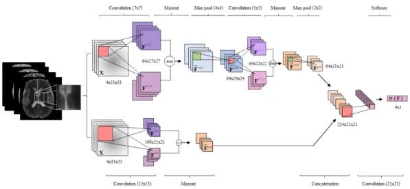
As mentioned earlier this network is a two-branch CNN based on the work by [4]. The branch with smaller 7×7 receptive field is called Local −
pathway and another with larger 13×13 receptive field is called Global −
pathway. This allows the prediction to be influenced by the high resolution details of the neighborhood around that pixel and its larger context i.e. overall location in the brain. The local pathway has two hidden layers which allow for the concatenation of both branches The concatenated feature maps are then fed to the fully connected layer.The full architecture along with its details is illustrated in Figure 1.1
Chapter 2
2.1
Implementation Details
The available BRATS data is split into Training Data (80% of the total data) and Validation Data (20% of the total data). The network is implemented in python using tensorflow-gpu.
Training is done in two phases to over-come the data imbalance between the different segmentation classes. In Phase 1 (P1) a uniform distribution over all the classes is assumed and the patches are generated accordingly. In Phase 2 (P2) the unbalanced nature of data is accounted for by assuming a more realistic distribution of data and training only the last layer of the network
2.1.1 Pre-processing
The raw images can be noisy, have bias field artifacts, motion artifacts, as well as other anatomy like eyes and skull. The BRATS data is already skull-stripped therefore we don’t apply any skull-stripping. The data is normalized to an intensity range of [0,1] within each modality (channel) by subtracting the channel’s mean and dividing by the channel’s standard deviation. The images of different subjects are then affinely registered using the T1 modality. The resulting transformation is applied to the remaining images.
2.1.2 Patch Extraction
Before training, 4D patches are extracted from the given MRI images to create training and validation data. the patch extraction is in accordance to the two phase training
Uniform distribution Equal number of patches from all segmenta-tion classes are extracted and a total of 1.8 mil patches are used for training in the first phase.
High Entropy For the second phase of training we sample from the regions of brain with multiple classes and class boundaries. Since such regions have high entropy we use an entropy filter. For each pixel in the input im-age the filter outputs the entropy value of a d×d neighborhood around the corresponding pixel, the entropy is calculated using:
S=−X
i
Pilog2Pi (2.1)
wherePi is the probability that the difference between the values of two adja-cent pixels isi.
Training on these patches allows the network to learn segmentation bound-aries more effectively. In addition to having a high entropy these patches are distributed similar to the natural frequencies of the classes (in the data) which removes a lot of false positives.
2.1.3 Hyper-parameter selection and tuning
Hyper-parameters refer to variables within the model that can not be directly learned from the training process. Defined in [1] as“hyper-parameter for a learning algorithm A is a variable to be set prior to the actual applica-tion of A to the data, one that is not directly selected by the learning algorithm itself ”
This tuning process is a meta optimization task that runs on top of loss op-timization. The hyper-parameters in this model include learning rate (α), momentum coefficient (β) and the L1 and L2 regularization coefficients (λ1 ,
λ2).
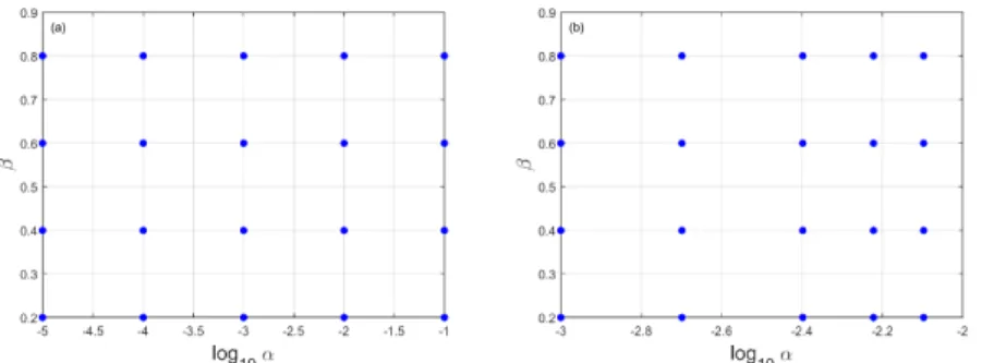
Learning rate and Momentum: α is arguably the most important hyper-parameter that needs to be tuned. A good approximation is to use a value close to the largest learning rate that doesn’t cause the training loss to diverge. For this purpose uniform grid search is used on G with increasing resolution after every full sweep see Figure 2.2
G={(α, β) :α ∈(1×10−5,1×10−1), β∈(0.2,0.8)} (2.2) The results are shown in Figure 2.3
Figure 2.2: Sampled values from uniform grid G(a) Coarse Grid (b) Fine Grid
L1 and L2 regularization coefficients: Selecting a suitable value forλ1 and λ2 (weight regularization co-efficeints) is not an easy task. A
com-mon practice is to use Grid Search to explore possible values between (0,1). Since the co-efficeints are regularizes its important to select their value based on their performance on out of sample data to compare generalization capabil-ities. For this purpose Cross Validation is used to select the best performing pair.
Figure 2.3: Tuning (α,β) (a) Coarse grid (b) Fine grid.
2.1.4 Training
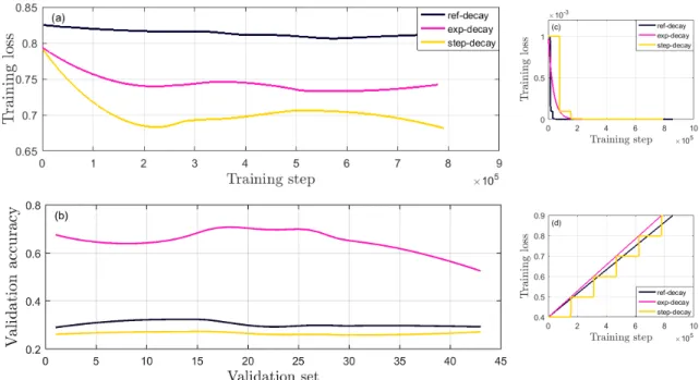
The number of training iterations is restricted by early stopping. The learning rate is decayed and momentum is gradually increased over the course of training. The reference strategy for adapting (α,β) is compared with two other schedules. Results are shown in Figure 2.5 and best performing method on validation set is used
step-decay: αe=α rbGlobalstepDecaystepc and β is step-wise increased to 0.9 (2.3)
exp-decay: α=α rGlobalstepDecaystep and β is gradually increased to 0.9 (2.4)
wherer is the decay rate and is set to 0.1
Figure 2.5: (a) Training results for different adaptive methods. (b) Validation accuracy of each method. (c) Learning rate decay schedule. (d) Momentum increase schedule
2.2
Results
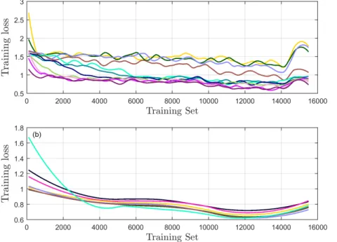
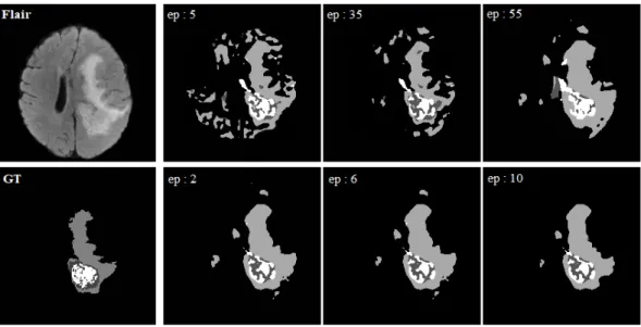
The network is trained for 55 epochs for P1 and 10 epochs for P2 .
Figure 2.6: Training results for Phase-1 (top) and Phase-2 (bottom) for different epochs
Segmenting one brain MRI with the trained model takes 1-2 minute. Figure 2.6 shows the improvement in prediction as the model undergoes training in both phases. Figure 2.7 shows the best validation prediction among the out of sample data.
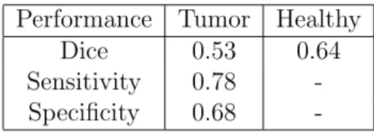
Typical measures of performance areDice,Sensitivity and Specif icity. Sensitivity measures the probability of a true positive i.e. the proportion of tumorous voxels that are correctly identified.
Specificity measures the probability of a true negative i.e. the proportion of healthy voxels that are correctly identified.
Performance Tumor Healthy
Dice 0.53 0.64
Sensitivity 0.78 -Specificity 0.68
-Table 2.1: Summary of results on validation data.
2.3
Conclusion
A fully convolutional deep neural network has been implemented suc-cessfully. It yields promising results however several issues remain open. The sensitivity and specificity values show that even though the model manages to correctly identify the tumor it is also prone to false positives.
The use of a convolution layer instead of the dense fully connected layer for output reduces both training and testing times. The data set containing 3.4 mil patches (2.2 mil healthy, 1.2 mil tumorous) was trained (1 epoch) in 1hr 40 minutes. For testing on a trained model it took 1-2 minutes to fully segment the 3D MR image.
Bibliography
[1] Yoshua Bengio. Practical recommendations for gradient-based training of deep architectures. CoRR, abs/1206.5533, 2012.
[2] Ezequiel Geremia, Bjoern H. Menze, Olivier Clatz, Ender Konukoglu, An-tonio Criminisi, and Nicholas Ayache. Spatial decision forests for ms lesion segmentation in multi-channel mr images. InProceedings of the 13th Inter-national Conference on Medical Image Computing and Computer-assisted Intervention: Part I, MICCAI’10, pages 111–118, Berlin, Heidelberg, 2010. Springer-Verlag.
[3] Ian J. Goodfellow, David Warde-Farley, Mehdi Mirza, Aaron Courville, and Yoshua Bengio. Maxout networks. In Proceedings of the 30th International Conference on InterInternational Conference on Machine Learning
-Volume 28, ICML’13, pages III–1319–III–1327. JMLR.org, 2013.
[4] Mohammad Havaei, Axel Davy, David Warde-Farley, Antoine Biard, Aaron C. Courville, Yoshua Bengio, Chris Pal, Pierre-Marc Jodoin, and Hugo Larochelle. Brain tumor segmentation with deep neural networks. CoRR, abs/1505.03540, 2015.
[5] B. H. Menze, A. Jakab, S. Bauer, J. Kalpathy-Cramer, K. Farahani, J. Kirby, Y. Burren, N. Porz, J. Slotboom, R. Wiest, L. Lanczi, E. Gerstner, M. A.
Weber, T. Arbel, B. B. Avants, N. Ayache, P. Buendia, D. L. Collins, N. Cordier, J. J. Corso, A. Criminisi, T. Das, H. Delingette, . Demi-ralp, C. R. Durst, M. Dojat, S. Doyle, J. Festa, F. Forbes, E. Geremia, B. Glocker, P. Golland, X. Guo, A. Hamamci, K. M. Iftekharuddin, R. Jena, N. M. John, E. Konukoglu, D. Lashkari, J. A. Mariz, R. Meier, S. Pereira, D. Precup, S. J. Price, T. R. Raviv, S. M. S. Reza, M. Ryan, D. Sarikaya, L. Schwartz, H. C. Shin, J. Shotton, C. A. Silva, N. Sousa, N. K. Sub-banna, G. Szekely, T. J. Taylor, O. M. Thomas, N. J. Tustison, G. Unal, F. Vasseur, M. Wintermark, D. H. Ye, L. Zhao, B. Zhao, D. Zikic, M. Prastawa, M. Reyes, and K. Van Leemput. The multimodal brain tumor image seg-mentation benchmark (brats). IEEE Transactions on Medical Imaging, 34(10):1993–2024, Oct 2015.
[6] Nitish Srivastava, Geoffrey Hinton, Alex Krizhevsky, Ilya Sutskever, and Ruslan Salakhutdinov. Dropout: A simple way to prevent neural networks from overfitting. J. Mach. Learn. Res., 15(1):1929–1958, January 2014. [7] Nagesh K. Subbanna, Doina Precup, D. Louis Collins, and Tal Arbel.
Hi-erarchical probabilistic gabor and mrf segmentation of brain tumours in mri volumes. In Kensaku Mori, Ichiro Sakuma, Yoshinobu Sato, Chris-tian Barillot, and Nassir Navab, editors, Medical Image Computing and
Computer-Assisted Intervention – MICCAI 2013, pages 751–758, Berlin,
Heidelberg, 2013. Springer Berlin Heidelberg.
Auto-matic brain tumor segmentation using cascaded anisotropic convolutional neural networks. CoRR, abs/1709.00382, 2017.