Essays at the Intersection of Environment and Development Economics

(1)

Essays at the Intersection of Environment

and Development Economics

The Harvard community has made this

article openly available.

Please share

how

this access benefits you. Your story matters

Citation

Walker, Elizabeth Ruth. 2015. Essays at the Intersection of

Environment and Development Economics. Doctoral dissertation,

Harvard University, Graduate School of Arts & Sciences.

Citable link

http://nrs.harvard.edu/urn-3:HUL.InstRepos:17467372

Terms of Use

This article was downloaded from Harvard University’s DASH

repository, and is made available under the terms and conditions

applicable to Other Posted Material, as set forth at

http://

nrs.harvard.edu/urn-3:HUL.InstRepos:dash.current.terms-of-use#LAA

(2)

Essays at the Intersection of Environment and

Development Economics

A dissertation presented by

Elizabeth Ruth Walker

to

The Department of Public Policy

in partial fulfillment of the requirements for the degree of

Doctor of Philosophy in the subject of Public Policy Harvard University Cambridge, Massachusetts April 2015

(3)

(4)

Dissertation Advisor: Professor Rema Hanna

Author: Elizabeth Ruth Walker

Essays at the Intersection of Environment and Development Economics

Abstract

The three essays in this dissertation explore how households in Southern Africa interact with and rely upon environmental resources. The first chapter examines the relationship between irrigation dam placement and local infant health outcomes. Irrigation dams can enable farms to harness considerable water resources, and this has been critical to increasing the global food supply. However, irrigation consumes 70 percent of global water resources and returns polluted water back into river systems. I examine the effect of irrigation dams on water pollution and infant health outcomes in South Africa. To remove bias associated with non-random dam placement, I utilize an instrumental variables approach that predicts dam placement using geographic features and time-varying policy changes. I find that each additional dam within a district increases both water pollution and infant mortality. In districts downstream from dams, alternately, dams generate smaller water pollution effects and reduce infant mortality, though magnitudes are much smaller. I argue that this pattern is consistent with pollution-induced health costs that outweigh economic benefits within the districts that receive dams. Downstream, however, pollution generates smaller costs and the economic benefits dominate. Exploring other plausible channels through which irrigation dams may affect infant mortality, I find that while irrigation dams generate substantial effects on district employment and small effects on migration, these factors do not appear to explain the health outcomes observed. Instead, the results suggest that water pollution and reduced water availability may contribute to higher infant mortality near agricultural activity.

The second chapter in this dissertation explores technology adoption of trees with environ-mental benefits, in the context of a field experiment in Zambia. As context, many technology adoption decisions are made under uncertainty about the costs or benefits of following through

(5)

with the technology after take-up. As new information is realized, agents may prefer to aban-don a technology that appeared profitable at the time of take-up. Low rates of follow-through are particularly problematic when subsidies are used to increase adoption. This chapter uses a field experiment to generate exogenous variation in the payoffs associated with taking up and following through with a new technology: a tree species that provides fertilizer benefits to adopting farmers. Our empirical results show high rates of abandoning the technology, even after paying a positive price to take it up. The experimental variation offers a novel source of identification for a structural model of intertemporal decision making under uncertainty. Estimation results indicate that the farmers experience idiosyncratic shocks to net payoffs after take-up, which increase take-up but lower average per farmer tree survival. We simulate coun-terfactual outcomes under different levels of uncertainty and observe that subsidizing take-up of the technology affects the composition of adopters only when the level of uncertainty is relatively low. Thus, uncertainty provides an additional explanation for why many subsidized technologies may not be utilized even when take-up is high.

Finally, the third paper in my dissertation explores the role that mineral wealth has on local economic outcomes. Mineral wealth has been central to the development of the South African economy. However, we have little evidence regarding how it has affected employment and poverty. This paper explores how within-country variation in mineral wealth affects district-level outcomes. Using data on mineral deposits and historical world prices, I construct a plausibly exogenous variable reflecting district-level aggregate mineral wealth, and I use variation in this index to evaluate economic outcomes over three Census rounds (1991, 1996, 2001). In the short run, I show that positive shocks to aggregate mineral wealth generate higher employment, largely driven by increased mining employment. This increase in mining is accompanied by reductions in agricultural employment and slight reductions in manufacturing employment. On average, adult age individuals also report working more hours and earning higher salaries in districts experiencing higher mineral prices. In sum, mineral wealth shocks generate benefits to districts, with less households below the poverty line.

(6)

List of Tables

1.1 Geographic Characteristics of All and Former Homeland Districts . . . 16

1.2 Mother Characteristics and Instrument Test . . . 21

1.3 The Effect of River Gradient on Dam Construction (First Stage) . . . 22

1.4 The Effect of Dam Construction on Infant Mortality . . . 24

1.5 Robustness Checks using Additional Controls . . . 26

1.6 Other Health Outcomes . . . 28

1.7 District-Level Water Quality Changes . . . 30

1.8 Probability of Exceeding WQ Standards Downstream from Dams . . . 32

1.9 Household Outcomes Related to Changes in Water Source . . . 34

1.10 Employment Outcomes in Response to Dams . . . 36

1.11 Average District Migration Statistics (1996 to 2001) . . . 39

1.12 Profile of In-migrants and Out-migrants . . . 41

2.1 Summary Statistics . . . 70

2.2 Comparison of Structural and Reduced Form Estimates . . . 72

2.3 Structural Parameter Estimates . . . 83

3.1 List of Mineral Deposits . . . 109

3.2 Cross-Section Relationship between Deposit and District Characteristics . . . 117

3.3 The Effect of Five-Year Price Shock on District Employment and Poverty . . . 119

3.4 The Effect of Five-Year Price Shock on District Employment and Poverty, by Major/Minor Minerals . . . 122

3.5 The Effect of One-Year Price Shock on Individual Employment and Poverty (1995-1999) . . . 123

3.6 Quartile Regression of District Employment on Income Shocks . . . 124

A.1 Irrigation Dam Summary Statistics . . . 138

A.2 Descriptive Statistics of Chemical Indicators . . . 140

A.3 Infant Mortality Results by Type . . . 147

A.4 District-Level Changes (First Difference) . . . 149

A.5 Employment Outcomes by Gender . . . 151

(10)

B.1 Stochastic Tree Survival . . . 166

B.2 Knowledge and Experience with the Technology . . . 168

B.3 Procrastination . . . 169

B.4 Incentive Spillovers within Group . . . 170

B.5 Balance . . . 171

B.6 Attrition Across Data Collection Phases . . . 172

B.7 Correlation Between Farmer Observables and Program Outcomes . . . 173

(11)

List of Figures

1.1 Map of Former Homeland Areas . . . 10

1.2 Map of Dam Locations and Average River Gradient by District . . . 13

1.3 Example of Data . . . 14

2.1 Take-up and Follow-through Thresholds as a Function of Agent Type . . . 56

2.2 Experimental Design . . . 63

2.3 Farmer Expected Profit as a Function of Uncertainty . . . 88

2.4 Take-up and Threshold Outcomes as a Function of Uncertainty . . . 90

2.5 Tree Survival as a Function of Uncertainty . . . 91

3.1 Average Value of the Instrument Across Districts . . . 115

3.2 Variation in Minerals Price Index within South Africa . . . 116

A.1 Dams in Africa as of 2007 . . . 137

A.2 Dam Construction by Year and Purpose . . . 137

A.3 Percent Homeland Area in Each Magisterial District . . . 142

(12)

Acknowledgments

I am incredibly grateful to the people that supported me throughout my PhD.

This dissertation would not have been possible without the guidance and encouragement of my advisors Rema Hanna, Rob Stavins, Rohini Pande and Kelsey Jack. Their mentorship made my PhD an enjoyable, productive and deeply rewarding learning experience. In particular, I am thankful for Rema’s incredible patience, technical direction and life advice as I produced my job market paper; for Rob’s mentorship on how to teach a great economics class; for Rohini’s guidance on how to make research policy-relevant; and for Kelsey’s help in connecting research to theory and her practical advice on performing field experiments.

Many colleagues and friends also generously took the time to help me during the disser-tation process, including Chris Avery, Bill Clark, Nancy Dickson, Ariel Stern, Rich Sweeney, Sara Lowes, Megan Bailey, Martin Abel, Deanna Ford and the participants in the Harvard Environmental Economics and Development lunches. I am also grateful to Kelsey, Paulina Oliva, Sam Bell, Jonathan Green, and our team in Zambia for their collaboration on our field experiment. Nicole Tateosian and Jason Chapman also were very supportive, and kept me organized and productive.

For financial support, I am grateful to the Vicki Norberg-Bohm Fellowship, the Crump Fellowship, and the Jennifer Perini and Jim Cunningham Dissertation Fellowship. I am grateful for the assistance of the South Africa Department of Water Affairs, particularly Dr. Michael Silberbauer who provided data, insights and support.

For keeping me happy and sane, I thank my running girlfriends for thousands of miles over the last six years. For love and inspiration, I thank my family Dan, Kitty, Maria, Katie and Jay.

(13)

(14)

Chapter 1

Irrigation Dams, Water and Infant

Mortality: Evidence from South Africa

1.1 Introduction

Water is integral to food production, withdrawing 70 percent of global water resources (FAO, 2005). However, as agriculture intensifies in fast-growing, high food-demand regions of China, India, and Sub-Saharan Africa, growing concerns related to agricultural water use and human health may be warrented (e.g., Tilman et al., 2002; Seckler, 1999). Specifically, agricultural intensification increases yields but relies on water-consuming irrigation techniques and water-polluting agrichemical inputs. Estimating the effects of intensified agriculture on health outcomes is therefore instructive to designing policies that account for these potentially costly health externalities.

Empirically, linking agricultural water pollution to health outcomes is difficult, given that pollution originates from private, non-point sources. Moreover, households near polluted water sources may be systematically different from those further away, and increased pollution may alter behaviors or induce migration (Chay and Greenstone, 2003). As a consequence, most well-identified evidence of the causal effects of water pollution on health focuses on observable improvements to water infrastructure, such as switching from unprotected to protected springs (Kremer, 2011) or from natural to piped water (Jalan and Ravallion, 2003; Galiani et al., 2005).

(15)

Only a handful of recent papers incorporate data on surface water quality in order to identify plausibly causal relationships between water pollution and health outcomes (Ebelstein, 2012; Brainerd and Menon, 2014).

This paper builds on the existing literature by investigating a new and important channel: the effect of irrigated agriculture on infant mortality. South Africa is water stressed, and agriculture uses 60 percent of country-wide water resources, compared to 10 percent for urban and domestic use (CSIR, 2010; Oberholster and Ashton, 2008). I use the construction of irrigation dams as a proxy for agricultural water use and estimate the effect of an increase in irrigation dams on infant mortality. Irrigation dams, which henceforth I refer to as “dams,” are a useful indicator of intensive water use in this context, where low, erratic rainfall and depressed groundwater levels often make dam construction a primary means for increasing yields (Blignaut et al., 2009). The dams are predominantly small, privately owned, and constructed to support commercial agriculture. Moreover, South Africa has more dams than any other country in Africa, and the number more than doubled between 1980 and 2010, to

over 3,000 dams (Dam Safety Office, 2013).1

Estimating responses to new dam construction is confounded by non-random dam place-ment. On the one hand, governments or firms may target locations that are agriculturally more productive, growing faster, or politically better connected than those that do not receive dams. Alternately, dams may be situated in lower functioning districts to spur growth or expand production. As a result, a simple comparison of districts that receive dams with those that do not may be biased by other factors affecting outcomes. To control for endogenous dam placement, I adopt a variation of the approaches in Pande and Duflo (2007) and Strobl and Blanc (2013). I instrument for dam placement by interacting two sources of variation: spatial differences in river gradient suitability for dams and policy changes which affected

dam placement over time.2 _{I also present and discuss OLS estimates with fixed effects, which}

demonstrate the same pattern.

The instrumental variables (IV) estimation relies on shifts associated with Apartheid, the 1_{See Figure A.1 and Figure A.2.}

(16)

political system in place until 1994. Apartheid policies removed millions of black South Africans to marginal “homeland” regions. Dams were rarely constructed within or near homelands until after Apartheid. Thus, the IV strategy interacts a river gradient variable with a step variable reflecting the increasing likelihood that dams were placed in former homelands. This restricts the identification to variation within districts that are politically, economically and geographically more similar. In other words, the IV compares outcomes within former homeland districts that had river gradients more desirable for dams to those with steeper, less desirable river gradients, while controlling for district-specific geographic characteristics.

Restricting the IV analysis to responses within former homelands has three empirical

advantages. First, evaluating outcomes within former homelands enables plausibly separating the water-induced health effects from those caused by direct chemical exposure associated with working on plots sprayed with agrichemicals. In South Africa, mechanization during the 1950s drastically reduced agricultural labor to a subset of higher-skilled managers (Platsky and Walker, 1985). As of 2001, less than ten percent of the population was involved in agriculture, and in the former homelands less than one percent participated (Census, 2001). Second, the former homelands are more similar to other developing countries in Africa, where many households rely on surface and ground water. This makes the results more applicable to these similar countries. Finally, households within homelands were less able to migrate, which reduces the probability of differential migration driving results.

Given its dual effects on economic productivity and the environment, the effect of

dam-induced irrigation on infant mortality isa prioriambiguous. Economically, dams affect income

through improved labor opportunities and changes to local markets. Even if households are not directly involved in agriculture, there are likely to be increased post-production labor opportunities within the district. Evidence on small irrigation dams in South Africa finds that these dams generate small increases in crop production within districts (Strobl and Blanc,

2013).3 _{New labor opportunities could either reduce infant mortality by increasing household}

3_{This is in contrast to the research on large dam construction in India and Africa, which suggests that large} dams reduce agricultural production within a district while increasing it downstream (Duflo and Pande, 2007; Strobl and Strobl, 2010). Large dams are those at least fifteen meters in height or three million cubic meters in volume. For large dams, the channel through which productivity losses arise is somewhat different. In India, Duflo and Pande suggest that productivity losses arise as a result of community displacement and soil salinity. In

(17)

income or increase infant mortality through reductions in time spent caring for the child. A less considered channel is the concurrent water-related changes that arise as a result of dam-induced irrigation. Irrigation reduces water availability and increases water pollution within districts. Household responses to water-related changes depend on their ex ante water source, with those that rely directly on nearby rivers or groundwater being most vulnerable. Households should unambiguously switch water sources or migrate in response to pollution or low water availability, but this behavior change may be attenuated if pollution is unobservable, if households are unaware of possible adverse effects, or if marginal willingness to pay for improved water sources is low (Kremer et al., 2011; Greenstone and Jack, 2014). Evidence also suggests household characteristics, such as education and income, influence household choices and outcomes in response to water pollution (Jalan and Ravallion, 2003; Kremer et al., 2011).

Despite limited causal evidence, the water channel may be important. Empirical public health research suggests an observable correlation between agricultural water pollution and birth defects in the United States (Croen et al., 2001; Winchester et al., 2009). Building on this, recent causal research from India links agrichemical exposure to increases in poor infant and child health outcomes (Brainerd and Menon, 2014). However, in India, unlike South Africa or the United States, over half of the labor force is involved in agriculture, which means direct agrichemical exposure may contribute to results. Given that dams reduce water availability, research by Field et al. (2011) is also relevant. Using a natural experiment from Bangladesh, the authors estimate that infant and child mortality increase as a result of lower water availability and switching to farther water sources. Finally, within South Africa, countless government reports and news articles document deteriorating water quality and water availability (e.g.,

DEAT, 2006; Blaine, 2013; UN Water, 2011).4

This paper measures the net impact of dams on infant mortality, which includes the

combined effect of economic, environmental, and other unobservable channels. I find that South Africa, the data includes dams over five meters in height and the average surface area of constructed dams is 0.465 square km. This is much smaller than the average district area of 3,500 square km. As a result, population displacement by dams is less concerning.

4_{For example, a United Nations report estimates that river pollution, namely nutrient enrichment from} agriculture and acidity from industry, has left nearly two-thirds of freshwater species at risk of extinction in South Africa (UN Water, 2011).

(18)

each additional dam leads to an average 6 percent increase in infant mortality, off an already high average infant mortality of 4.8 percent. This result is in line with research demonstrating that various types of water pollution and variation in water sources significantly affect infant mortality.5

I then examine plausible channels through which dams may affect health. First, I show that newly constructed dams increase water pollution, as observed using chemical indicators. For example, average nitrate concentrations increase almost 50 pecent and other related indicators have smaller but significant increases of 3 percent to 11 percent. In addition, nitrate and total dissolved salt levels are significantly more likely to exceed drinking water standards downstream from new dams. The results corroborate existing case-based research from South Africa showing that small irrigation dams cumulatively reduce water flow and generate concentrated water pollution (e.g., O’Keeffe et al., 1990; O’Connor, 2001; Mantel et al., 2010).

To shed light on other channels, I evaluate employment and migration changes after Apartheid. New dams generate employment, despite falling national employment. While employment rates for men are almost double those for women, dam construction induces slightly greater employment gains for women. This could affect infant health if female caregivers are less attentive to infants. However, stratifying the sample by age demonstrates that employment gains are small for women under 30 and near zero for women over 50, the two age segments most likely to be primary caregivers. Finally, I investigate migration to ensure that selective out-migration is not altering district compositions in a way that could generate the observed infant mortality result. I show that in-migrants are more likely to have piped water, at least a high school education, and an income above the poverty line. These factors are unlikely to increase district infant mortality. Still, out-migrants have similar characteristics. To rule out that this influences the outcome, I show that dam construction does not alter average district characteristics significantly between 1996 and 2001.

This paper contributes to the empirical literature on the determinants of pollution and the 5_{For examples of papers linking water to infant mortality, see Clay et al. (2010) for lead water pollution, Galiani} et al. (2005) for transition to piped water sources, Cutler and Miller (2005) for water filtration/chlorination, Field et al. (2011) for switching to less convenient water sources, and Brainerd and Menon (2014) for agrichemical water pollution.

(19)

effects of pollution on health. Most estimates of infant health outcomes in response to pollution exposure focus on air pollution, both in the developed world (e.g., Chay and Greenstone, 2003; Currie and Walker, 2011) and developing world (e.g., Borja-Aburto et al., 1997; Jayachandran, 2009; Arceo-Gomez et al., 2012). There are far fewer estimates relating infant health to water pollution given lack of water quality data, the difficulty in obtaining precise estimates from water samples, and the fact that developed countries have long had nearly universal access

to clean drinking water sources (as discussed in Olmstead, 2009).6 _{This paper contributes}

new evidence that in places with limited water availability and insufficient water treatment infrastructure, there may be a direct trade-off between agricultural intensification and infant health.

The paper is divided into seven sections. Section 1.2 provides background on irrigated agriculture, water, infant mortality, and the South African context. Section 1.3 describes the data sources. Section 1.4 presents the empirical strategy, Section 1.5 describes results and Section 1.6 explores alternative channels. Section 1.7 concludes.

1.2 Background

In this section, I first describe the link between irrigated agriculture and water quality. Next, I discuss the relationships between water and infant health outcomes. Finally, I provide relevant institutional and policy details.

1.2.1 Irrigated Agriculture and Water Quality

In South Africa, semi-arid environmental conditions make commercial agriculture highly reliant on dams. On average, South Africa receives 500 mm of rain per year, much lower than the global average of 860 mm per year. This rainfall is highly variable and spatially concentrated in the east, falling on only 14 percent of arable land (Davies et al., 1995). Groundwater is also a small portion of water use, given low groundwater levels and recharge rates (Hughes, 2004; CSIR, 6_{Historical estimates, however, imply that the direct human health benefits of improved drinking water quality} are sizable: for example, Cutler and Miller (2005) estimate that introducing water disinfection in U.S. cities accounted for three-quarters of the decline in infant mortality during the early twentieth century.

(20)

2010). Dams hedge water-related risk and ensure enough water to irrigate crops. While total yields generated from irrigated agriculture are unknown, commercial agriculture generates 95 percent of total output in monetary terms and irrigated crops contribute substantially to this output (FAO, 2005).

Irrigated agriculture alters water systems in three ways that are important to health. First, irrigation dams siphon water from rivers and transport it via canals to irrigate crops. Some portion of the water is consumed by crops or evaporates, and some returns back to river

systems.7 _{While this regulates water flow in irrigation channels, it reduces water flow and}

availability to households downstream.8 _{Second, irrigation dams increase standing water,}

which can act as a breeding ground for mosquitos and increase vector-borne infections. Third, water return flows are often contaminated with fertilizer nutrients and pesticides (e.g., Tredoux et al., 2001; Walmsley, 2003). Agrichemical pollution will be exacerbated when total water is reduced.

Changes in water quality can be measured using chemical indicators, which reflect nutrient content and overall quality. Nitrate, phosphate and potassium are the primary components of fertilizer and the indicators most associated with agricultural pollution. Fertilizer run-off also increases total dissolved salts (National Assessment Report, 2002). In South Africa, fertilizers that contain gypsum will lead to elevated sulfate levels as well (Huizenga, 2011).

1.2.2 Water and Infant Mortality

Both water pollution and reduced water access can generate adverse health outcomes.9 _First,

existing evidence from the United States demonstrates a correlation between agricultural water pollution and birth defects, the leading cause of infant mortality in this context (e.g., Winchester et al., 2009). Both fertilizer nutrients and pesticides have been linked to developmental defects.

7_{Estimating how much water is consumed by crops rather than returned to the water system is difficult, given} its dependence on the rate of evapotranspiration, weather/season, crop types, and other factors. A global average suggests that 70 percent of water removed from rivers for agriculture is consumed by the water system (Cosgrove and Rijsberman, 2000; Shiklomanov, 1999).

8_{For examples, see O’Keeffe et al. (1988), O’Connor (2001), or Mantel et al. (2010).}

9_{Although the outcome measure is infant mortality, early life outcomes can be indicative of broader community} health and of health impacts that arise later in life. See Almond and Currie (2010) or Currie and Vogl (2012).

(21)

For example, high nitrate concentrations may directly induce infant mortality through “blue

baby syndrome.”10 _{Similarly, various pesticides have been associated with adverse fetal and}

infant health (e.g., Munger, 1992; Garry et al., 1996). Fertilizer nutrients, particularly when combined with slow flowing water, also cause toxic algal growth. Toxic algae pose a serious threat to several water streams in South Africa (e.g., van Ginkel, 2011; Oberholster, 2009). Toxic algae can cause infant death when ingested. Alternately, observable algae may induce households to seek other water sources (WHO, 2009).

Reduced water access prevents households from exercising appropriate hygiene. Water is necessary for hand washing, food preparation, and maintaining toilets. Without water, water-borne and water-washed diseases (e.g., trachoma, scabies, shigella) are more likely. Furthermore, lack of water leads caregivers to devote more time to searching and collecting water and less time to children. For these reasons, lower water usage can increase infant mortality (Pruss et al., 2002). The effect of unreliable water access on infant health is huge: the Millennium Development Goals document that lack of safe drinking water, open defication, and poor hygiene contribute an estimated 88 percent of all deaths for children under the age of five (2007).11

South Africa is an important context in which to study water and infant health. At 50 out of 1000 births, infant mortality in South Africa during the 1990s was ten times that found in developed countries. Babies may be vulnerable to infant mortality given mother characteristics and the high HIV/AIDs prevalence. For example, only 66 percent of infants from former homeland districts were delivered in hospitals and only 45 percent were breastfed within the first hour of life. Moreover, relying on breast milk exclusively is rare. While most mothers breastfed their infant at least once, only seven percent exclusive breastfeed in the first six months. This is important because mortality from environmental factors is more likely after 10_{Blue baby syndrome arises because nitrate ingestion leads to decreased oxygen carrying capacity in the blood.} Infants under six months are particularly susceptible to this condition, given low levels of the enzymes required to reverse this condition (Knobeloch et al., 2000). Evidence suggests this outcome is rare (Fewtrell, 2004), but does occur. See also Manassaram (2006) or Avery (1999) for reviews of the literature on nitrates and infant health outcomes.

11_{The weights of different health channels are unknown, given the difficulty in isolating them (e.g., as discussed} in Hunter, 2010).

(22)

children are weened from breast milk (Esrey et al., 1991). Given that the median age of infant death is five months in this sample, exposure to environmental hazards could contribute to mortality.

1.2.3 Institutional and Policy Context

Between the 1950s and the 1970s, several policy shifts forced millions of black South Africans

into independent homelands, yieldingde factosegregation and limited mobility.12 _{Water rights}

were assigned with land rights, which were reserved for whites (Rose, 2005). The ethnic homelands were fragmented resettlement zones on the rural outskirts of productive regions, as shown in Figure 1.1. The homelands negotiated with the government for rights to water and were underserved as a result. Rivers were a primary domestic water source for many households (Funke et al., 2007). When the first democratic government was elected in 1994, the homelands were incorporated into existing provinces and the government made efforts to remove biases against dam placement in former homelands.

12_{The homelands were 13 percent of land area but approximately 40 to 50 percent of the total population as of} the 1990s (Anderson, 2005; Thompson, 2001).

(23)

Figure 1.1:Map of Former Homeland Areas

The pink regions reflect former homeland areas under Apartheid. The homeland areas were integrated back into South Africa after the first democratic government was elected in 1994. The analysis relies on magisterial district boundaries (the black lines).

More formal policy, laid out in the National Water Act of 1998, nationalized water rights. As a result of the government transition and reforms, millions gained access to improved water sources. Despite increased access to improved water sources, competitive water pricing in the 1990s kept prices high. As of 1995, about 20 percent of households used river water as their primary domestic source, though more used it as a secondary source.

Despite improvements, twenty-seven percent of households reported inadequate water supply during 1995 and 1996. Furthermore, even piped water sources sometimes retain pollution from natural sources. Government reports document non-functioning treatment

facilities as a serious problem, in some cases increasing pollution levels because of poor

practices (e.g., CSIR, 2011; Igbinosa, 2009; Silverbauer, 2009). Agricultural runoff is regulated, but regulations are difficult to enforce.

(24)

1.3 Data

In this section, I discuss the data sources utilized for this analysis. Additional details regarding the data are provided in the Appendix.

1.3.1 Dam and Hydrological Data

The dam data was collected from the Dam Safety Office within the Department of Water Affairs. All dams that stand at least 5 meters in height and 50,000 cubic meters in capacity are required to register with the Dam Safety Office. The dataset provides information on the dam owner, designer, catchment area, surface area, wall type, wall height, drainage area, main purpose(s), contractor, wall height, capacity, GPS coordinates, spillway area, catchment area, and completion date for dams. Eighty percent of constructed dams report a purpose of “irrigation” and I restrict the data to these. In 1980, 131 districts (37 percent) had no dams and 83 districts (23 percent) had over five dams. By 2010, only 89 districts (25 percent) had no dams and 147 districts (43 percent) had greater than five.

As shown in Table A.1, less than five percent of dams report multiple purposes. Ninety-five percent of dams in the data are embankment dams, constructed using compacted earth materials to create a water barrier. Water is stored behind the wall in a reservoir and can be transferred nearby using canals. Embankment dams rely on gravity-based flow, thus a gentle gradient ensures enough slope for water flow. However, slope increases velocity, which in turn increases soil erosion and sedimentation. Soil erosion creates cloudy water, suffocates riverbed ecosystems and erodes downstream canals, among other negative consequences. As a result, steep gradients are undesirable for irrigation dams, which I exploit in the identification.

I also utilize water quality and river network data from the South Africa Department of Water Affairs. The water quality data is collected by the National Monitoring Programme and includes 1,672 monitoring stations. Monitoring began as a way to ensure irrigation viability, but today monitors water quality for climate change, domestic use, agriculture, and industry. Most stations had one reading per station per month, which I use to construct station-month-year averages and district-year averages. For the main analysis, I restrict the data to only stations in

(25)

place as of 1990, in order to avoid biases associated with new stations being placed in response

to poor pollution.13 _{Although homeland areas were underserved under Apartheid, about 25}

percent of stations existed in these districts. Descriptive statistics of chemical indicators are shown in Appendix Table A.2. As the table shows, South African water quality is already poor, with about 10 percent of readings for several indicators above drinking water standards.

To construct the river gradient instrument, I use a complete mapping of the river network from the Department of Water Affairs. About 50 percent of rivers flow perennially, with the rest seasonal/dry (35 percent) or unknown (15 percent). I extract perennial river segments,

given that dams are more likely to be placed on these rivers (Strobl and Blanc, 2013).14 _{For the}

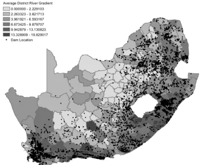
subset of river pixels within the district, I match river pixels to land gradient data and calculate the fraction of river pixels which are steep, defined as greater than six percent slope. Figure 1.2 demonstrates that dams are concentrated in areas with gentle to moderate, rather than steep, river gradients.

13_{The results are robust to alternative methods of collapsing the data, including using the means, using only} stations with at least seven years of data, and trimming the data (removing top and bottom 1%).

14_{Dams can be constructed on seasonal rivers, but it is less likely given unpredictable flow. I also control for} total river length (seasonal and perennial) in the instrumented regressions.

(26)

Figure 1.2:Map of Dam Locations and Average River Gradient by District

Average District River Gradient 0.000000 - 2.229103 2.263323 - 3.821713 3.961921 - 6.593167 6.673425 - 9.879707 9.942879 - 13.130823 13.328909 - 19.829017 Dam Location

Each dot on the map indicates the location of a dam. Most irrigated grain agriculture is concentrated on the eastern side of the country.

I coded the upstream/downstream relationships among districts based on the direction of flow for each river that crossed a district boundary. Each river segment contains an order code, which increases as a river flows downstream. I rely on this, but verify it using elevation changes along the river. In Figure 1.3, for example, three districts have rivers that flow into the main district, thus there are three upstream districts. In cases where two districts had rivers going in both directions, I marked these district pairs as adjacent and do not include them in the current analysis.

(27)

Figure 1.3:Example of Data Tarka Elliot Lady Frere Engcobo Molteno Cala Cofimvaba Wodehouse Sterkstroom Queenstown Indwe Tsomo Hewu Nqamakwe Ntabethemba Maclear Hofmeyr Idutywa Steynsburg Cradock _Cathcart Barkly East Albert

The above figure is a snapshot of the data. The turquoise line is the outline of one district in the sample, Lady Frere. The black lines reflect district boundaries, the black dots indicate dams, and the dark blue lines are the river network. For larger dams, I have the polygon locations, shown in light blue. The surface area of dams in this setting tends to be a small fraction of the total district area.

1.3.2 Survey Data

I pool three rounds of infant birth and death data from the Demographic and Health Surveys. The survey was collected in 1987, 1998, and 2003 and aims to be nationally representative of women between the ages of 15 and 49. I construct a record of child births and deaths based on the detailed fertility history provided by women in the sample. Mothers report the date of

birth for each child, whether the child died, and if so, the date of death.15 _{In the data, each}

child birth becomes an observation, and I construct an indicator that equals one if the child died within the first year of life. This provides an estimate of child mortality for a given year. This generated a dataset of 31,807 births and deaths, spread over 22 years.

Household-level data from The October Household Survey (OHS) allows me to further 15_{For the 1987 survey, I only use data on the last two children born, given this data is considered most accurate} (Phillips, 1999).

(28)

explore behavioral responses to dams. The nationally-representative surveys were conducted to inform post-Apartheid reconstruction and development, and the surveys are similar to the World Bank Living Standards Measurement Surveys. The survey asks questions related to access to water and use of different water sources. It also asked labor-related questions, including employment, hours worked, and salary.

Finally, I utilize the more comprehensive 10 percent population sample of the 1996 and 2001 Census to evaluate migration patterns in response to dams. The limitation with Census data is that I cannot construct a panel given only two rounds of reliable information.

1.3.3 Districts as Unit of Analysis

I link geographic and survey data sources using the magisterial district boundaries that were in place before the end of Apartheid. Magisterial boundary data was obtained from Global Administrative Boundaries. Although boundary re-demarcation occurred several times after Apartheid, I rely on spatial coordinates of subsequent survey enumeration areas to match

each survey round with the former boundary areas.16 _{There were 354 magisterial districts in}

South Africa. A magisterial district has an area of about 3,500 square km. Across districts, the population grew from about 82,000 people per district in 1980, to 126,000 people per district in 2000.

To construct former homeland districts, I match homeland maps to magisterial district maps. I define districts that had at least 30 percent former homeland area as a “homeland” district. A map of homeland areas, shown in Figure 1.1, confirms that homelands tended to be concentrated in a subset of all districts. This fact is confirmed in Figure A.3. Because most districts had either no homeland area or a significant portion, the main results hold across different cut-off values. Table 1.1 also demonstrates that homelands tend to be steeper, drier, and more densely populated. Thus, they were somewhat less likely to receive dams, though many are still constructed during the period of my analysis.

16_{For some survey data, the former magisterial district is recorded at the time of surveying. This served as a} check on the matching.

(29)

Table 1.1: Geographic Characteristics of All and Former Homeland Districts

Variable All Districts_Mean Homelands_Mean

(1) (2)

Fraction of River Gradient Pixels 0-1.5% 0.294 0.197

[0.202] [0.173]

Fraction of River Gradient Pixels 1.5-3% 0.22 0.189

[0.088] [0.093]

Fraction of River Gradient Pixels 3-6% 0.189 0.211

[0.079] [0.070]

Fraction of River Gradient Pixels > 6% 0.286 0.392

[0.233] [0.244] District Elevation 1.016 817 [498] [424] District Slope 9.14 11.88 [6.26] [6.29] River Length (km) 569.35 418.19 [936.68] [457.42]

District Population (1996 Census) 103,696 149,632

[126,858] [89,299]

Number of Districts 354 100

Notes:

1. Each observation reflects one district. The first column includes all districts. The second column is only former homeland districts.

2. The means for all districts are reported in column (1), and the means for only former homeland districts are reported in column (2). Standard deviations reported below in brackets.

3. The geographic variables were constructed using ArcGIS, and the population was estimated using the 10 percent sample of the 1996 Census.

(30)

1.4 Identification Strategy

1.4.1 Instrumental Variables

The analysis is designed to measure the effects of irrigation dams on health outcomes. If irrigation dam placement is randomly assigned, then the following regression identifies the relationship between dams and outcomes:

yidt =go+g1Ddt+g2DdtU+yeart+ddt+ld+#idt (1.1)

where yidt is the outcome of interest for observationiin districtdand yeart. The variable

Ddt is the cumulative number of operational dams in the district as of yeart, andDU_dt is the

cumulative number of operating dams in all upstream districts.17 _{The remaining right hand}

side variables control for unobservable heterogeneity: year fixed effects, district-level trends, and district fixed effects.

As discussed above, this strategy is biased, given that dams are possibly placed in locations that are systematically different from other locations along dimensions that are difficult to entirely control for in a regression framework. If factors that affect dam construction are also likely to affect infant mortality, this generates correlation between the true error term and

the dam coefficient, resulting in a biased estimate of g1, the effect of an additional dam on

health outcomes in that district. The direction of the bias depends on which factors drive dam placement. For example, dams are more likely to be placed in areas with growing agriculture, industry, or resources, and newly constructed dams are accompanied by improvements in

access to food, health or labor opportunities, theng1will be lower or more negative, as dams

reduce infant mortality.

Instead, I instrument for dam construction. First, I construct a variable that denotes the fraction of steep river gradient pixels within a district (greater than six percent slope). To generate time-varying predictions, the steep river gradient variable is interacted with a variable 17_{I also consider the possibility that dams have nonlinear effects on outcomes. The residuals of the regression} above are roughly normally distributed (both with and without trends). I also perform the analysis using logs and using quadratic terms, both of which reasonably describe the data. These results available by email.

(31)

reflecting dam placement policies. After Apartheid ended and the Water Act was enacted, nationalized water policy favored dam placement broadly (Strobl and Blanc, 2013). To denote this, I create a step function that gives former homeland districts a value of 0 prior to 1994, 1 from 1994 to 1997, and 2 from 1998 to 2010. As a result, the policy variable is an interaction

between a location (former homeland area), denoted H_d, and a year, denoted At. I interact

time-invariant river gradient with the time-varying policy variable, HdAt. This yields the

following first stage:

D_dt= bo+b1(Steepd⇤Hd⇤At) +b2(Xd⇤Hd⇤At) + (Steepd⇤yeart) +Hd⇤At+gp+#dt (1.2)

where Ddt equals the cumulative number of dams in districtd and yeart, and Steepd is

the fraction of river pixels that have a steep gradient (greater than 6 percent).18 _{I also include}

geographic controls,Xd, including sum of all seasonal and perennial rivers, district elevation

categories (0-500 m, 500-1000 m, >1000 m) and district gradient categories (1.5-3%, 3-6%, and >6%). I interact the geographic controls with the policy variable to allow the effect of each control to vary with the policy shifts. The steep river gradient-year interaction term allows for the time-varying shocks, like weather or new technologies, to affect steep river gradients differentially. I also control for district or province fixed effects,gp.19

The first stage predicts the number of dams in the district and the number of dams upstream

from the district.20 _{The second stage equation uses these predicted values to estimate health}

outcomes:

18_{Previous versions of this paper used a combination of three river gradient instruments, based on different river} gradient slopes (similar to Pande and Duflo, 2007). However, for the small dams in this setting, a single variable -steep river gradient - is sufficient to predict dam placement.

19_{In all cases except infant mortality, I use district fixed effects. Given that infant mortality is a low probability} event and the number of observations is limited, I rely on province fixed effects and fraction homeland controls (in addition to all geographic controls).

20_{To predict}d_DU

dtusing equation (2), I take the sum of all the upstream predicted dams. For controls, I use the

average of upstream districts for variables that enter as averages (elevation, slope, percent homeland) and the sum for variables that enter cumulatively (river length).

d DU dt = dDU1 + dD2U + DdU3 + DdU4 = bo + b1 ⇣ Steepup_d 1H_dup1Aup_t 1⌘ + b2 ⇣ Steepup_d 2H_dup2Aup_t 2⌘ + b3 ⇣ Steepup_d 3H_dup3Aup_t 3⌘+b4 ⇣

(32)

yidt=go+g1Dddt+g2dD_dtU+g4Zd+g5ZUd +#idt (1.3)

where dD_dt is the number of dams predicted in the district, dDU

dt is the number of dams

predicted upstream,Zd is the set of district-level controls, andZU_d is the set of controls for the

upstream district. The outcome variable,yidt, is infant mortality in the primary analysis, and

then other outcomes in subsequent analysis (water quality, water source, and employment variables). In each case, the IV regression captures the local average treatment effect of dams. In other words, the estimated coefficient,g1, reflects the average effect of each additional dam

on districts that receive dams as a result of river gradient desirability.

In the results that follow, I report both IV and OLS coefficients. While the regressions are run on the same observations, the coefficients for the two specifications rely on somewhat different observations for the identification. In the OLS specifications, I use district and year fixed effects for the entire country. Therefore, the coefficient on dams and upstream dams in the OLS represents a reduced-form relationship: the correlation between number of dams and the outcome variable. For the main outcomes, I also show the interaction of dams with homeland district, which identifies the additional effect of dams within homelands. This is more similar to the IV coefficient, which captures the effect of an additional dam within homeland districts over time.

1.4.2 Threats to Identification

The exclusion restriction requires that the instrument only affects outcomes via its effect on the likelihood of irrigation dam construction. This exclusion restriction criteria fails if the

instrument is independently correlated with the outcome, after conditioning on covariates.21 _In

this case, the covariates are critical. For example, districts may have received preferential access to electricity after the end of Apartheid, and this is correlated with land gradient (Dinkelman, 2011). I control for this using land gradient-policy interactions. Another possible threat to 21_{Note that the river gradient component of the instrument can and is itself correlated with at least one outcome} variable, water quality. But, in those regressions I control for district fixed effects. The results are not causal if changes in the policy variable (Pdt=HdAt) differentially affect water quality by river gradient.

(33)

the identification is the Land Reform Act enacted to assist in land redistribution toward the poor. However, this is more likely to be targeted based on land gradients (which I control for) and only two percent of land had been redistributed as of 2001 (Twala, 2006; Strobl and Blanc, 2013).

Furthermore, the instrument compares differences in dam constructionwithin homeland

areasover time. Thus, even if policies across homeland and non-homeland areas were quite different, it will not affect estimates within homeland areas. This does assume that even if dam or water-related policies varied within former homeland areas, the design and enforcement of these policies was not systematically different based on the river gradient. In other words,

absent dam construction, changes in infant mortality would not have variedby river gradient

within homeland areas.

1.5 Results

1.5.1 Balance and First Stage

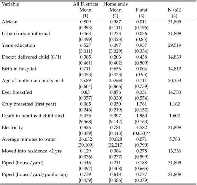
Table 1.2 presents summary statistics for the mothers in the sample. Column (1) includes all mothers in South Africa and column (2) restricts the sample to mothers within former homelands. Across all districts, mothers are poor, tend to live in rural areas, do not have piped

water, and travel about 30 minutes to obtain water.22 _{In the third column, I regress each mother}

characteristic on the steep river gradient variable, with geographic controls. This test provides supporting evidence that the river gradient instrument is uncorrelated with most mother characteristics. The exception is electricity.23 _{Given that the instrument relies on variation over}

time, the IV assumption remains valid so long as outcomes do not vary differentially by river gradient as policy changes.

22_{A caveat to this table is that the responses are reported as of the time of survey, not at the time of the child’s} birth. This is a limitation of the data.

23_{Given fourteen variables were tested, finding at least one significant variable is expected with a ten percent} threshold.

(34)

Table 1.2: Mother Characteristics and Instrument Test

Variable All Districts Homelands

Mean Mean F-stat N (all)

(1) (2) (3) (4) African 0.809 0.987 0.011 31,809 [0.393] [0.111] (0.196) Urban/urban informal 0.463 0.233 0.036 31,809 [0.499] [0.423] (0.85) Years education 6.527 6.097 0.937 29,519 [3.011] [3.029] (0.334)

Doctor delivered child (0/1) 0.305 0.203 0.438 14,839

[0.461] [0.402] (0.509)

Birth in hospital 0.711 0.656 0.004 14,812

[0.453] [0.475] (0.95)

Age of mother at child’s birth 25.89 25.968 0.111 30,153

[6.604] [6.866] (0.739)

Ever breastfed 0.85 0.876 0.351 14,733

[0.357] [0.330] (0.554)

Only breastfed (first year) 0.065 0.050 1.781 1,162

[0.246] [0.219] (0.152)

Death in months if child died 5.475 5.397 1.960 1,602

[9.568] [9.142] (0.163)

Electricity 0.826 0.781 4.582 31,809

[0.379] [0.413] (0.033)**

Average minutes to water 26.632 30.028 0.071 5,783

[30.109] [32.217] (0.790)

Moved into residence <2 yrs 0.129 0.084 0.278 13,336

[0.336] [0.277] (0.599)

Piped (house/yard) 0.446 0.211 0.188 31,809

[0.497] [0.408] (0.665)

Piped (house/yard/public tap) 0.739 0.618 0.777 31,809

[0.439] [0.486] (0.379)

Notes:

1. Each observation reflects a child’s mother in the sample. Mothers may be present more than once if they had multiple children in the sample. The data was pooled across three rounds of survey data. For the variables with N between 13,000 - 15,000, only the 1998 and 2003 rounds were available. For the "only breastfed" variable, only those born in the last year and in the 1998 survey round were available.

2. The table reports the means for all districts in column (1) and the means for only former homeland districts in Column (2). Standard deviations reported below in brackets.

3. Column (3) regresses the mother variable on the steep river gradient variable, with geographic controls. I test whether the steep river gradient variable is significant and I present the F-test, with p-value in parentheses.

4. Asterisks denote significance: *** p<0.01, ** p<0.05, * p<0.1.

(35)

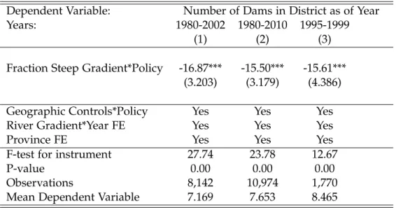
The first stage is presented in Table 1.3 for each subset of years used in the analysis. The instrument is the fraction of steep river gradient pixels interacted with changes in Apartheid policies in Homeland districts. In all specifications, the F-statistic suggests that the instrument is strong.

Table 1.3: The Effect of River Gradient on Dam Construction (First Stage)

Dependent Variable: Number of Dams in District as of Year

Years: 1980-2002 1980-2010 1995-1999

(1) (2) (3)

Fraction Steep Gradient*Policy -16.87*** -15.50*** -15.61***

(3.203) (3.179) (4.386)

Geographic Controls*Policy Yes Yes Yes

River Gradient*Year FE Yes Yes Yes

Province FE Yes Yes Yes

F-test for instrument 27.74 23.78 12.67

P-value 0.00 0.00 0.00

Observations 8,142 10,974 1,770

Mean Dependent Variable 7.169 7.653 8.465

Notes:

1. Each observation reflects a district-year combination. The dependent variable is the number of irrigation dams constructed as of that district-year. 2. Each column reports the results of estimating equation (2) for the subset of years for which infant mortality, water quality, and household data are available. The term "Policy" refers to the interacted variable (H*A).

3. The controls including the following geographic variables, each interacted with the policy variable (H*A): total length of seasonal and perennial rivers, total district area, district slope category (0-1.5%, 1.5-3%, 3-6%, >6%), district elevation category (0-500 m, 500-1000 m, >1000 m). The regression also controls for the main effect of the policy variable (H*A), steep gradient*year fixed effects, and province fixed effects.

4. Robust standard errors clustered at the district level are in parentheses for the panel. Asterisks denote significance: *** p<0.01, ** p<0.05, * p<0.1. 5. The data source for the dam data is the Department of Water Affairs.

1.5.2 Infant Mortality

Table 1.4 shows the IV and OLS results for the effect of irrigation dams on infant mortality. The estimates capture the combined effect of irrigation dams on infant health, inclusive of all

(36)

changes arising from markets, the environment and any omitted variables. Columns (5) and (6) present the IV result using estimating equation (3) and show large positive coefficients on irrigation dams in the district. The coefficient (.003) is approximately a six percent increase on

the dependent mean infant mortality (0.048).24 _{In addition to estimating the IV using two-stage}

least squares, I present the results using limited information maximum likelihood, given this estimation method is more robust to weak instruments (Stock and Yogo, 2005).

24_{These estimates are consistent with the literature. Brainerd and Menon (2014) estimate that a 10 percent} increase in average fertilizer chemical concentrations during the month of conception raised infant mortality likelihoods by 4.6 percent. Galiani et al. (2005) estimate reductions in under-5 child death of 5-8 percent associated with privatization. Field and Glennester (2011), alternatively, found that when households switched from closer arsenic-contaminated wells to further away wells or surface water sources, infant and child mortality increased 27 percent.

(37)

Table 1.4: The Effect of Dam Construction on Infant Mortality

Dependent Variable: Infant Death

Type of Regression: OLS OLS OLS Logit (w/FE) IV (2SLS) IV (LIML) (1) (2) (3) (4) (5) (6) Dams in District 0.00218* 0.00158* 0.000805 0.0685*** 0.00309** 0.00313** (0.00113) (0.000947) (0.00101) (0.0210) (0.00134) (0.00137) Dams Upstream 0.000288 0.000249 0.00132*** 0.00705 -0.000813* -0.000826* (0.000334) (0.000291) (0.000440) (0.00682) (0.000488) (0.000496) Dams in District* Homeland (0.00288)0.0104*** Dams Upstream* Homeland -0.00168** (0.000665)

District FE Yes Yes Yes Yes Year FE Yes Yes Yes Yes Province-Year Trends Yes

Geo. Controls*Policy Yes Yes River Gradient*Year FE Yes Yes

Province FE Yes Yes

First Stage F-Statistic 51.94 51.94 Observations 31,809 31,809 31,809 29,366 31,809 31,809 Mean Dep. Variable 0.048 0.048 0.048 0.052 0.048 0.048 Notes:

1. Each observation reflects a single birth from 1980-2002. The outcome variable equals zero if the child is alive at one year, and one if the child has died within the first year.

2. Columns (1) through (4) report the regression of infant mortality on number of dams in the district and number of dams upstream, with controls as reported. Column (3) interacts the dam coefficients with a binary variable indicating former homeland. Column (4) reports the results of a logit regression using conditional fixed effects.

3. Columns (5) and (6) report the results using the instrument. For these specifications, the following control variables are included, each interacted with the policy variable: total length of seasonal and perennial rivers, total district area, district slope category (0-1.5%, 1.5-3%, 3-6%, >6%), district elevation category (0-500 m, 500-1000 m, >1000 m), and fraction homeland category. For upstream dams, I control for the same variables: average upstream slope, average upstream elevation, total upstream river length, and total upstream district area. The regression also controls for the main effect of the policy variable (H*A), steep gradient*year fixed effects, and province fixed effects.

4. The F-Statistic is the Cragg-Donald Wald F-Statistic.

5. Robust standard errors clustered at the district level are reported in parentheses. Asterisks denote significance: *** p<0.01, ** p<0.05, * p<0.1.

6. The infant mortality data is from the South Africa Demographic and Health Surveys (1987, 1998, 2003).

(38)

The OLS estimates, which rely on fixed effects, provide corroborating evidence that dams increase infant mortality. These estimates control for district and year fixed effects in column (1), and district and year fixed effects with a province time trend in column (2). While the trends absorb some variation, the effect size remains positive and significant at the 10 percent level. In column (3), I re-run the OLS specification interacting the dam variable with an indicator for being a former homeland district. I find that the interaction is positive, suggesting that dams are correlated with relatively higher infant mortality increases within former homelands. This is unsurprising, given that households within homelands were more disadvantaged than the average household and mothers in former homelands were more likely to rely on river water

sources.25 _{This result is similar to the IV result, which looks at the effect size within former}

homelands. The OLS somewhat overestimates the effect of dams on infant mortality, which could suggest that dams are placed in areas that are experiencing lower growth or declining health.

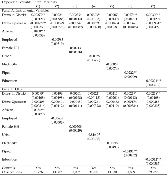
Downstream, dams generate net reductions in infant mortality, at least in the IV. However, estimated coefficients are an order of magnitude smaller than those within the district and the estimates are not statistically different from zero in the OLS. While net impacts are small, the IV results suggest that districts downstream from dams experience net health benefits greater than costs. The small effects of upstream dams are as predicted, given the small size of dams. In Table 1.5, I check that the increase in infant mortality is robust to the inclusion of mother controls. The controls are characteristics reported by the mother at the time of surveying, not at the time of the child’s birth. Because some of the mother controls may be endogenous, the regression coefficients for the characteristics cannot be easily interpreted. However, the controls should be correlated with the characteristic at the time of child birth. Thus, this table provides some confidence that the estimated effects are robust to the inclusion of household characteristics. Unfortunately, the mother characteristics are not asked in every survey round; for that reason, columns (2), (3) and (5) are smaller samples.

25_{Because infant mortality is a binary variable, I also present conditional logit with district and year fixed effects} in column (4). The average marginal effect from the conditional logit regression is much larger at the mean, given it is bounded (0/1). However, it is useful to check that it remains positive.

(39)

Table 1.5: Robustness Checks using Additional Controls

Dependent Variable: Infant Mortality

(1) (2) (3) (4) (5) (6) (7)

Panel A: Instrumental Variables

Dams in District 0.00272** 0.00224 0.00239* 0.00303** 0.00207 0.00274** 0.00300** (0.00121) (0.000985) (0.00144) (0.00133) (0.00139) (0.00131) (0.00129) Dams Upstream -0.000772** -0.000579 -0.000540 -0.000795 -0.000404 -0.000678 -0.000931* (0.000350) (0.000776) (0.000589) (0.000488) (0.000583) (0.000485) (0.000492) African 0.0400*** (0.00553) Employed -0.00583 (0.00519) Female HH 0.00243 (0.00426) Urban -0.00378 (0.00466) Electricity -0.00867 (0.00574) Piped -0.0222*** (0.00399) Education -0.00291*** (0.000612) Panel B: OLS Dams in District 0.00195* 0.00196 0.00201 0.00221* 0.00211 0.00219* 0.00218** (0.00108) (0.00198) (0.00198) (0.00113) (0.00201) (0.00113) (0.00108) Dams Upstream 0.000208 -0.000401 -0.000450 0.000261 -0.000483 0.000174 0.000288 (0.000316) (0.00112) (0.00111) (0.000328) (0.00110) (0.000334) (0.000335) African 0.0354*** (0.00479) Employed -0.00458 (0.00503) Female HH 0.000508 (0.00429) Urban -9.81e-07 (0.00406) Electricity -0.00719 (0.00491) Piped -0.0191*** (0.00432) Education -0.00312*** (0.000585)

Controls Yes Yes Yes Yes Yes Yes Yes

Observations 31,726 13,082 13,087 31,809 13,030 31,809 29,227

Notes:

1. Each observation reflects a single birth from 1980-2002.

2. The IV regression includes the following control variables, each interacted with the policy variable: total length of seasonal and perennial rivers, total district area, district slope category (0-1.5%, 1.5-3%, 3-6%, >6%), district elevation category (0-500 m, 500-1000 m, >1000 m), and fraction homeland category. For upstream dams, I control for the same variables: average upstream slope, average upstream elevation, total upstream river length, and total upstream district area. The regression also controls for the main effect of the policy variable (H*A), steep gradient*year fixed effects, and province fixed effects.

3. The OLS regressions include for district and year fixed effects.

4. Employment, female household head and electricity questions were not available for the 1987 round, so the regression has a smaller sample.

(40)

This version of the paper assumes no health spillovers to adjacent districts. This assumption is generally reasonable, given that districts are large and operate as roughly separate labor markets (as discussed in Dinkelman, 2011). In addition, pollution is unlikely to travel further than the district. However, it is possible that dams affect adjacent districts through one or several channels. For example, water for irrigation is transferred in some instances and could affect results. In this case, the result would provide a conservative estimate of the effect of dams on health.

1.5.3 Other Health Outcomes

Evidence of water-related illnesses in response to dams provide support for the health-water channel. To evaluate this, I rely on mother responses to other health-related questions in the DHS data. In each survey round (1987, 1998, 2003), mothers are asked about the health of their children in the last two weeks.26 _{In Table 1.6, I present evidence that children in districts}

which receive more dams experience more fevers, coughs and diarrhea in the last two weeks. All three outcomes could indicate greater water-related illness. Fevers indicate any infection, including malaria, which is predicted to increase in response to stagnant water (EPA, 2014; WHO, 2014). Similarly, coughing can indicate respiratory illness. Finally, infants consuming polluted water or in households with low water access are more likely to experience diarrhea, though the effect is imprecise and not statistically distinguishable from zero.

26_{I restrict the sample to children under five years of age, given this is all that was surveyed in 2003 round. In} the 1987 survey, the responses are further restricted to the last two children born into the household.

(41)

Table 1.6: Other Health Outcomes

Dependent Variable: Fever in the

last two weeks last two weeksCough in the last two weeksDiarrhea in last two weeksDiarrhea in (_2 yr old)

(1) (2) (3) (4)

Panel A. Instrumental Variables

Dams in District 0.0518*** 0.0606*** 0.0124* 0.0134 (0.0131) (0.0228) (0.00691) (0.0110) Dams Upstream 0.00808 0.0230 -0.00437 -0.0289*** (0.0151) (0.0194) (0.00989) (0.00991) Panel B. OLS Dams in District 0.00611** 0.00600** -0.00175 -0.00423 (0.00255) (0.00287) (0.00181) (0.00351) Dams Upstream 0.000176 0.000435 0.00117 0.00209 (0.000837) (0.00108) (0.000958) (0.00151)

Controls Yes Yes Yes Yes

Observations 32,315 29,315 29,311 9,619

Mean Dep. Variable 0.113 0.125 0.066 0.133

Notes:

1. Each observation is a living child age 5 or younger, surveyed in one of three rounds of DHS data (1987, 1998, and 2003). The analysis is restricted to "currently living" at the survey time, but the results look the same if deceased children are included.

2. The question in the survey asked whether the respondent had experienced one of the above conditions during the past two weeks.

3. The IV regressions include the following control variables, each interacted with the policy variable: total length of seasonal and perennial rivers, total district area, district slope category (0-1.5%, 1.5-3%, 3-6%, >6%), district elevation category (0-500 m, 500-1000 m, >1000 m), and fraction homeland category. For upstream dams, I control for the same variables: average upstream slope, average upstream elevation, total upstream river length, and total upstream district area. The regression also controls for the main effect of the policy variable (H*A), steep gradient*year fixed effects, and district fixed effects.

4. The OLS regressions include district and year fixed effects.

5. Robust standard errors clustered at the district level are reported in parentheses. Asterisks denote significance: *** p<0.01, ** p<0.05, * p<0.1.

6. Infant mortality data is from the South Africa Demographic and Health Surveys (1987, 1998, 2003).

(42)

1.6 Channels

I next evaluate several possible channels through which dams may affect infant mortality, including changes in water quality, water sources, employment and migration.

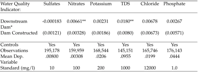
1.6.1 Water Quality

I first explore water quality responses to dams. Table 1.7 presents the results of the IV regression in Panel A and the OLS regression in Panel B. In Panel