A Continuous Optimization Model for Partial Digest Problem

A Continuous Optimization Model for

Partial Digest Problem

H. Salehi Fathabadi

*

and R. Nadimi

Department of Applied Mathematics, School of Mathematics, Statistics, and Computer Science, Faculty of Sciences, University of Tehran, Tehran, Islamic Republic of Iran

Received: 26 January2009 / Revised: 16 February 2010 / Accepted: 23 February 2010

Abstract

The pupose of this paper is modeling of Partial Digest Problem (PDP) as a

mathematical programming problem. In this paper we present a new viewpoint of

PDP. We formulate the PDP as a continuous optimization problem and develope a

method to solve this problem. Finally we constract a linear programming model

for the problem with an additional constraint. This later model can be solved by

the simplex method in which a restricted basis-entry-rule is defined.

Keywords: Molecular biology; Continuous optimization; Simplex method; DNA; PDP

*

Corresponding author, Tel.: +98-21-66412178, Fax: +98-21-66412178, E-mail: [email protected]

Introduction

One of the interesting tasks in computational biology is Restriction Site Mapping. When a particular restriction enzyme is added to a DNA, the DNA is cut at particular restriction sites. The goal of restriction site mapping is to determine the location of every site for a given enzyme. Using gel electrophoresis, one can find the distance between each pair of restriction sites. In the Partial Digest Problem (PDP), the distances arising from digestion experiments with one enzyme are given, and the locations of all restriction sites must be computed.

Let X = {x0,x1,...,xn} be the set of restriction site locations on a DNA strand. We denote the "multiset" of

all 1

2

n N = + 

  pairwise distances between these site

locations by ∆X ={xj−x xi| j>xi, ,i j = 0,1,..., }n .

Suppose that, in PDP, a multiset B = { ,b b1 2,...,b_N}

of distances is given. Our goal is to find a set

0 1

= { , ,..., n}

Y y y y of points on a line such that B is the

pairwise distance multiset of Y. We denote the

minimum and maximum of B by bm and bM,

respectively.

This problem was presented in the 1930's in the area of X-ray crystallography [1]. In 1988 P. Lemke and M. Werman, solved it by a pseudo-polynomial time algorith[2]. The running time of the presented algorithm

depends on bM. Skiena et al[3] suggested a backtracking

algorithm to solve the problem where its running time was depended only on n. In 1994, Z. Zhang, by an example, showed that the running time of backtracking algorithm in worst case is exponential [4]. Then, in

2000, T. Dakice in his Ph.D. thesis presented a 0 1−

quadratic programming model for PDP and solved it by a heuristic successive semidefinite programming algorithm [5]. Finally, in 2005, M. Cieliebak et al. proved that Partial Digest Problem is hard to solve for erroneous input data [6].

Modeling this problem using mathematical

optimization model that can be solved by the well-known simplex method with restricted entry rule for non-basic variables.

In Section 1, we introduce the continuous

optimization model for PDP. In section 2 the model is

converted to a linear programming problem with an additional set of constraints and dvelop an extended version of the simplex algorithm to solve the problem.

Continuous Optimization Model

Suppose that there are N = (n n+1) / 2 line

segments with lengths of b b1, 2,...,bN . We want to

place them in a line interval [0,bM] such that the

multiset of endpoints of these line segments equals to

1 2

= { , ,..., N}

B b b b . In other word, we are to provide a

solution of PDP with endpoints of line segments. Let a

line segment with length bj be denoted as "b -j

segment". It is obvious that the beginning point of bM

-segment is zero and its endpoint is bM . Let the

variables xj and xj+N , j = 1, 2,...,N show the

beginning and end points of bj-segment in the interval

[0,bM ], i.e. xj+N −xj =bj for all j = 1, 2,...,N .

We design an optimization model with

1 2 2

= { , ,..., N}

X x x x as the decision variables such that,

at optimality, X has exactly (n+1) different values

and the multiset of these values is equal to B . We

define the new set X by eliminating the replicated

members of X . (The number of different values in X

is equal to the cardinality of X , |X |).

Each set of values of xj's that are between zero and

M

b , and satisfy the constraints xj+N −xj =bj

,j = 1, 2,...,N , is defined as a "placement" of line segments b b1, 2,...,bN in interval [0,bM]. It is clear that a placement in which the number of its endpoints is not

equal to (n+1) is not desirable. Moreover, in the

following example, we show that it is possible to place

the line segments in interval [0,bM ] with (n+1)

endpoints such that the multiset of the endpoints is not

equal toB .

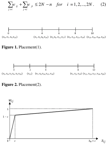
Example 1. let B = {2, 2, 2, 4, 4, 4, 6, 6,8,10} be the

input data of PDP. Then we haveN = 10, n= 4 and

the target interval is [0,10] . Also we have:

1= 2

b ,b2 = 2,b3= 2,b4= 4,b5= 4,b6 = 4,

7= 6

b ,b8= 6,b9= 8,b10 = 10.

Now we present two different placements of these

line segments in interval [0,10] with n+1 = 5

endpoints, such that one of them is a solution of PDP

but the other one is not. In the presented placement in

the Table 1 (placement(1)), X is equal to

{0, 4, 6,8,10} and ∆X is equal to B. Therefore, X is

a solution of PDP. In the placement(2), Table 2, X

is equal to {0, 2, 4,8,10} but ∆X = {2, 2, 2, 4, 4, 6,

6,8,8,10} is not equal to B and ,hence, X is not a

solution of PDP. _□

Review of differences between placement(1) and placement(2) is useful to provide the rule of correct

placing. In placement(1) for each xk from X there are

exactly n=4 members of X equal to xk (see Figure 1),

but in placement(2) only x13 is equal to 2 and there are

more than 4 members of X equal to 4 (see Figure 2).

In placement(2) some bj −segments coincide with

each other, i.e. they have the same beginning and end

points. For example b b4, 5 and b6 are coincided

together. But in placement(1) there is no coincidence. In the following lemma and theorem it is proved that

each placement of B with (n+1) different endpoints

that has no coincidence, is a solution of PDP.

Lemma 1. If a placement has no coincidence, then its

set of endpoints consists of at least (n+1) different

values.

Proof. If a placement X does not have any

coincidence, then each pair of members of X

corresponds at most to one member of B. Suppose that

X has r members. The number of distinct pairs of the

members is greater than or equal to N (N =|B|). This

means:

Table 1.xi's values of placement(1)

i 1 2 3 4 5 6 7 8 9 10

bi 2 2 2 4 4 4 6 6 8 10

xi 4 6 8 0 4 6 0 4 0 0

xi+10 6 8 10 4 8 10 6 10 8 10

Table 2.xi's values of placement(2)

i 1 2 3 4 5 6 7 8 9 10

bi 2 2 2 4 4 4 6 6 8 10

xi 8 8 0 0 0 0 4 4 0 0

(

1

)

1

2 2 2

n n

r + n+

   

≥ =

   

   

Therefore: r≥n+1_□

Theorem 1. Let X be a placement with no coincidence

and corresponding X has exactly (n+1) members,

then X is a solution of PDP.

Proof. In a placement with no coincidence each bj has

a unique corresponding pair (xk,xl), so that xk =xj

and xl =xj+_N . Therefore there are N distinct pair of

members of X corresponding to members of B. On

the other hand, there is only N members in ∆X ,

hence there is no member of ∆X that is not in B. That

is ∆X =B. _□

Now, in oredr to avoid coincidence, we define a set

of constraints in placing bj's. A coincidence occurs

when two line segments with the same length have equal beginning and end points. If we consider the following constraint in the placing process, then we have no coincidence in a placement:

= >

j i m j i

x −x ≥b if b b and j i (1)

Suppose that X is a placement for

1 2

= { , ,..., N}

B b b b . We use the term "ε-colony" to

present a subset of X such that distance between each

pair of it's members is less than ε. In other words, the

subset

1 2

= { l , l ,..., l_r}

S x x x is an ε-colony if

{ l_j l_i | , = 1, 2,..., } <

max x −x i j r ε. It is clear that if

<bm

ε , then there is no line segment placed in an ε

-colony. Moreover with respect to the constraints 1, if

<

ε { |

3

j i

j

b b

min − b >b i ji, , = 1, 2,...,N}, then for

each pair of ε-colonies S1 and S2, there is at most one

i

b such that xi ∈S1 and xi+N ∈S2. Therefore,

immediately, we have the next theorem:

Theorem 2. In a placement with respect to constraints 1,

if < { , { | > , , = 1, 2,..., }}

3

j i

m j i

b b

min b min b b i j N

ε − ,

then there are at least (n+1) ε-colonies such that the

distance between each pair of them is greater than ε._□

Now we constract an optimization model with X as

the set of decision variables so that, at optimality, the

corresponding X is a solution of PDP. We denote the

distance between xi and xj by zij, i.e.

=| |

ij i j

z x −x . To avoid duplication we define zij

only for j ≥i .

In order to complete the model we define an objective function and a set of constraints.These constraints and the objective function ensure that there

are exactly (n+1) different values for xj in the

optimal solution. Let’s define new variables

, , = 1, 2,..., 2 .,

ij

w i j N j ≥i which indicate the share of

ij

z ‘s in the objective function.

1

( ) ,

( ) (1 ) > .

ij ij

ij

ij ij

M

z if z w

z if z b

ε

ε ε

ε

ε ε ε

−



≤

 

=

 − + −



Figure 3 shows the curve of this function.

In the definition of wij , ε is a positive real value

less than 1 . When ε is much smaller than

M

b , the

gradient of the first segment of the curve is much steeper than the gradient of the second segment.

Using the following constraints, the next lemma shows that adding constraints (2) to the placing process

restricts the number of ε-colonies to (n+1).

> <

2 = 1, 2,..., 2 .

ij ji

j i j i

w + w ≤ N −n for i N

∑

∑

(2)

Figure 1. Placement(1).

Figure 2. Placement(2).

Lemma 2. If we choose < 1

2N n 1

ε

− + in any

placement that satisfies constraint (2), then each

neighbourhood Nε(xi) has at least n members for any

i, where Nε(xi)={ ||x x −xi |<ε}.

Proof. Suppose that there exist an index i such that

( i)

Nε x has less than n members. Then, there are at

least (2N −n+1) variables xj, such that zij =

|xi −xj |>ε, and:

> <

> (2 1)(1 )

ij ji

j i j i

w + w N −n+ −ε

∑

∑

or

> <

> (2 )

ij ji

j i j i

w + w N −n

∑

∑

which violate constraints 2. _□

With respect to Theorem 2 and Lemma 2, in any placement satisfying constraints (1) and (2) for

1

< { ,

2 1

min N n

ε

− +

{ | > , , = 1, 2,..., , ,1}

3

j i

j i m

b b

min − b b i j N b

we have exactly (n+1) ε-colonies such that each of

them has exactly n members. (The number of members

of X is 2N = (n n+1)).

Now we can state the complete model as follow: (P)

<

: = ij

i j

minimize f

∑

w

subject to:

1

( ) ,

=

( ) (1 ) > .

ij ij

ij

ij ij

M

z if z w

z if z b

ε

ε ε

ε

ε ε ε

−



≤

 

 _{− + −}



=| |

ij i j

z x −x for j > ,i i j, = 1, 2,..., 2N ,

=

j N j j

x + −x b for j = 1, 2,...,N ,

j i m

x −x ≥b for bj =bi, j > ,i i j, = 1, 2,..., 2N ,

> <

2

ij ji

j i j i

w + w ≤ N −n

∑

∑

for = 1, 2,..., 2i N ,

0≤xj ≤bM for j = 1, 2,..., 2N ,

= 0 N

x .

In problem(P), ε is a real number less than:

1

{ ,

2 1

min

N −n+

3

{ | > , , =1, 2,..., }, , }

3

j i M

j i m

M

b b b

min b b i j N b b n

−

+

Remember that the reasons for constraints, 1

<

2N n 1

ε

− + , ε <bm and < { 3 | > ,

j i

j i

b b min b b

ε −

, = 1, 2,..., }

i j N were discussed earlier. In the next

Theorem we show that the constraint < M ₃

M

b b n

ε

+ ,

(which yields ε< 1) implies that an optimal solution of

P, is a solution to the corresponding PDP.

Theorem 3. If 1 1 1

(X ,Z W, ) and 2 2 2

(X ,Z W, ) are two

feasible solutions of problem P such that 1

X is a

solution to the corresponding PDP and 2

X is not, then

we have:

1 1 1 2 2 2

( , , ) < ( , , )

f X Z W f X Z W

Proof. Let (X Z W, , ) be an arbitrary feasible solution

of P. Any feasible solution of P satisfies constraints 1

and 2. Therefore there are exactly (n+1) ε-colonies

such that each of them has exactly n members. We

denote these ε-colonies by [ ] , = 1, 2..., (x i i n+1) and

their length by δi, = 1, 2..., (i n+1).

Each pair ([ ] ,[ ] )x r x l ( > )l r of these ε-colonies

defines a unique bj in B, so that xj∈[ ]x r and

[ ]

j N l

x + ∈ x . Let's Ij( )x , Ij( )x and Ij(X) are

defined as follow:

( ) = { || |< }, ( ) = { || |< }

j i j j i j N

I x i x −x ε I x i x −x + ε

( ) ={( , )| , j( ) ( ), > , > }

j j mn

I x m n m n I∈ x ∪I x z ε n m

It is clear that 2

|Ij( ) |=x n . Let the length of

colonies that include the beginning and end of bj be

denoted by δj and δj respectively, and define ˆδj as

follow:

ˆ =j j j

δ δ +δ

We split the objective function into f1 and f2 with

1 2 1 2

<

= , ( , , )= ij, ( , , )= ij

i j i j

z_ij z_ij

f f f f X Z W w f X Z W w

ε ε

< <

≥

+

∑

∑

Now compare the values of the objective function in

1 1 1

(X ,Z W, ) and 2 2 2

(X ,Z W, ). It is clear that for

each 2

( , )m n ∈Ij(x ) (j = 1, 2,L,N ), we have:

2 _ˆ2

mn j j

z ≥b −δ and for each 1

( , )m n ∈Ij(x ),

1

=

mn j

z b . Therefore:

2 1 2 2

2 1

( , ) ( ) ( , ) ( )

ˆ

( )

ij ij j

M

i j I_j x i j I_j x

w w n

b ε δ ∈ ∈ ≥ −

∑

∑

which implies

2 1 2 2

2 1

=1_{( , ) ( )} =1_{( , ) ( )} =1

ˆ

( )

N N N

ij ij j

j _{i j I x} j _{i j I x} j

M

j j

w w n

b ε δ ∈ ∈ ≥ −

∑ ∑

∑ ∑

∑

Now we have

2 2 2 1 1 1 2 2

1 1 =1 ˆ ( , , ) ( , , ) ( ) N j j M

f X Z W f X Z W n b

ε δ

≥ −

∑

On the other hand

1 2 2 =1 =1 ˆ ₌ N n j i j i n δ δ +

∑

∑

Hence 3 1

2 2 2 1 1 1 2

1 1 =1 ( , , ) ( , , ) n i i M n f X Z W f X Z W

b

ε δ +

≥ −

∑

(3)

Moreover

1 1 1

2( , , ) = 0

f X Z W

and

1

2 2 2 2 2

2 =1 2_< 1 1 ( , , ) = n ij i

i j i

z_ij

f X Z W z

ε ε ε δ ε ε + < − − ≥

∑

∑

Therefore 1

2 2 2 1 1 1 2

2 2 =1 1 ( , , ) ( , , ) n i i

f X Z W f X Z W ε δ ε

+ −

≥ +

∑

(4)

With respect to equations 3 and 4 we have

2 2 2 1 1 1

3 1 1

2 2 =1 =1 ( , , ) ( , , ) 1 n n i i i i M

f X Z W f X Z W n b ε ε δ δ ε + + ≥ − −

∑

+

∑

In order to complete the proof, it is sufficient to show

that 3 1 < M n b ε ε ε −

In problem P we assumed that < M ₃

M b b n ε + , therefore 3 1 < M M b n b ε + or : 3 1 < M n b ε ε −

According to < 1

2N n 1

ε

− + , ε is less than 1 and

3 1 < M n b ε ε ε − □

Result: If a PDP has a solution, the corresponding

model P has a feasible solution and the optimal

solution of P is a solution of PDP.

It should be mentioned that if PDP has any solution,

it has 2k

(for some integer k ) different solutions ,[6],

for which the value of the objective function in

corresponding P is the same for all of them.

Presenting a Ppiecewise Linear Programming Model

In the previous section we presented a continuous

optimization model for PDP. In this model wij ‘s are

nonlinear(piecewise linear) function ofzij’s. In this

section we convert this model to a linear programming

problem with an extra constraint. We write wij ‘s and

ij

z ‘s as convex combinations of the break points in

curve of wij’s.

If 0≤zij ≤ε , then there are

0

0 ij

λ ≥ and 1

0 ij

λ ≥

such that:

0 1

0 1 1

0 1 1

= 1

= 0 =

= 0 (1 ) = (1 )

ij ij

ij ij ij ij

ij ij ij ij

z w

λ λ

λ ελ ελ

λ ε λ ε λ

 +  +   + − − 

and if ε≤zij ≤ε+bM , then there are

1

0 ij

λ ≥ and

2

0 ij

1 2

1 2

1 2

= 1

= ( )

= (1 ) 1

ij ij

ij ij _M ij

ij ij ij

z b

w

λ λ

ελ ε λ

ε λ λ

 ₊



+ +

 

− +



These equations yield:

0 1 2 1 2

0 1 2 1 2

0 1 2

0 2

= 0 ( ) = ( )

= 0 (1 ) 1 = (1 ) 1

= 1

= 0

ij ij ij _M ij ij _M ij

ij ij ij ij ij ij

ij ij ij

ij ij

z b b

w

λ ελ ε λ ελ ε λ

λ ε λ λ ε λ λ

λ λ λ

λ λ

 + + + + +



 + − + − +

 

+ +

  

We substitute these results in problem P. Before

substitution, consider that with respect to the objective

function, the constraint zij =|xi −xj | is equivalent to

the following constraints:

0 0

ij j i

ij j i

z x x z x x

+ − ≥

 

− + ≥



After substitutions, we have a linear programming

problem with an additional set of constraints: 0 2

= 0 ij ij

λ λ .

We denote the new problem by P′.

(P′) 1 2

<

: = ((1 ) ij ij)

i j

minimize f

∑

−ε λ +λ

subject to:

1 2

( ) 0

ij bM ij xj xi

ελ + +ε λ + − ≥

for j > ,i i j, = 1, 2,..., 2N ,

1 2

( ) 0

ij bM ij xj xi

ελ + +ε λ − + ≥

for j > ,i i j, = 1, 2,..., 2N ,

=

j N j j

x + −x b for j = 1, 2,...,N ,

j i m

x −x ≥b

= , > , , = 1, 2,...,

j i

for b b j i i j N ,

1 2 1 2

>((1 ) ij ij) <((1 ) ji ji) 2

j i −ε λ +λ + j i −ε λ +λ ≤ N−n

∑

∑

= 1, 2,..., 2

for i N ,

0 1 2

= 1

ij ij ij

λ +λ +λ for j > ,i i j, = 1, 2,..., 2N ,

0 2

. = 0

ij ij

λ λ for j > ,i i j, = 1, 2,..., 2N ,

0 1 2

, , 0

ij ij ij

λ λ λ ≥ for j > ,i i j, = 1, 2,..., 2N ,

0≤xj ≤bM for j = 1, 2,..., 2N ,

= 0 N

x .

As in the problem (P), here ε is a real number less

than

1

{ ,

2 1

min

N −n+

3

{ | > , , =1, 2,..., }, , }

3

j i M

j i m

M

b b b

min b b i j N b b n

−

+ .

Problem(P′) could be solved by simplex method

with "restricted basis-entry-rule". In this rule, λij0 or

2

ij

λ

is introduced into the basis only if it improves the objective function and if the new basis has only one of

0

ij

λ or λij2 [1]. In [1], this method has been used for

obtaining an approximating solution to the separable programming.

Results

In this paper our goul was to construct and analyse an exact mathematical model of Partial Digest Problem and propose a proper algorithm to solve it. Hence, we developed a continuous optimization model, which is solvable by the simplex method with restricted basis-entry-rule. Theoretically the running time of the simplex method is exponential but, in practice, the simplex method works surprisingly well and exhibits linear

complexity; proportional to n+m where n and m are

the number of variables and constraints respectively in the problem. The computational complexity of Partial Digest Problem is an open problem. Neither a proof of NP-hardness nor a polynomial time algorithm is known for this problem. Mathematical programming models have a long history in optimization theory and there are many powerful methods to solve them. We hope this

model of PDP, open a new view to this problem.

References

1. Bazaraa M. S., Sherali H. D., and Shetty C. M.Nonlinear programming theory and algorithms, Second edition, p:512, John Wiley and Sons, Inc, (1993).

2. Cieliebak M., Eidenbenz S., and Penna P.Partial Digest is hard to solve for erroneous input data. Theor. Comput. Sci., 349(3): 361-381, (2005).

3. Dakic T., On the Turnpike Problem. PhD thesis, Simon Fraser University, (2000).

4. Lemke P., Werman M.On the complexity of inverting the autocorrelation function of a finite integer sequence, and

the problem of locating n points on a line, given the ( ) 2 n

unlabelled distances between them. Preprint 453, Institute for Mathematics and its Application IMA, (1988) 5. Patterson A. L. A direct method for the determination of

the components of interatomic distances in crystals, Zeitschr. Krist. 90: 517-542, (1935).

6. Skiena S. S., Smith W., and Lemke P. Reconstructing sets from interpoint distances. In Proc. of the 6th ACM Symposium on Computational Geometry (SoCG 1990), pages 332-339, (1990).

7. Zhang Z., An exponential example for a partial digest mapping algorithm. Journal of Computational Biology,