Fast Feature Selection for Naive Bayes Classification in Data Stream Mining

Fast Feature Selection for Naive Bayes

Classification in Data Stream Mining

Patricia E.N. Lutu

Abstract - Stream mining is the process of mining a

continuous, ordered sequence of data items in real-time. Naïve Bayes (NB) classification is one of the popular classification methods for stream mining because it is an incremental classification method whose model can be easily updated as new data arrives. It has been observed in the literature that the performance of the NB classifier improves when irrelevant features are eliminated from the modeling process. This paper reports studies that were conducted to identify efficient computational methods for selecting relevant features for NB classification based on the sliding window method of stream mining. The paper also provides experimental results which demonstrate that continuous feature selection for NB stream mining provides high levels of predictive performance.

Index terms - data mining, feature selection, Naïve Bayes

classification, stream mining

I. INTRODUCTION

Predictive data mining involves the creation of classification or regression models. A classification model predicts the value of a categorical dependent variable while a regression model predicts the values a numeric dependent variable. Data stream mining also known as stream mining is the process of mining a continuous, ordered sequence of data items in real-time [1], [2], [3]. Naïve Bayes (NB) classification is one of the popular classification methods for stream mining. The popularity of the NB classifier for stream mining stems from the fact that it is very easy to update the NB model for classification as new stream data arrives. It has been observed in the literature that the performance of the optimal Bayes classifier (from which the NB classifier is derived) is not affected by irrelevant features, that is, features with little or no predictive power. However, it has also been observed that the performance of the NB classifier improves when irrelevant features are eliminated from the modeling process. Since stream mining is done in real time, there is a need to employ fast methods of modeling.

This paper reports studies that were conducted to identify efficient computational methods for selecting relevant features for NB classification based on the sliding window method of stream mining. The paper also provides experimental results which demonstrate that continuous feature selection for NB stream mining provides high levels of predictive performance compared to once-off feature selection. The rest of the paper is organised as follows: Section II provides background for stream mining, Naïve Bayes classification and feature selection.

Manuscript received 25 March 2013; revised 14 April 2013. P. E. N. Lutu is a Senior Lecturer in the Department of Computer Science,

University of Pretoria, Pretoria 0002, Republic of South Africa, phone: +27124204116;fax: +27123625188; web: http://www.cs.up.ac.za/~plutu; e-mail: [email protected]

Section III presents the experimental methods. Section IV presents the experimental results. Section V concludes the paper.

II. BACKGROUND

A. Stream mining

Data collected over time is commonly described as a data stream. More precisely, a data stream is a real-time, continuous, ordered sequence of data items [1], [2], [3]. One major challenge for mining data streams is due to the fact that it is infeasible to store the data stream in its entirety. This problem makes it necessary to select and use training data that is not outdated for the mining task. The second challenge for stream mining is due to the phenomenon of concept drift, which is defined as the gradual or rapid changes in the concept that a mining algorithm attempts to model [1], [2], [3]. Given that data items arrive continuously and that the concept being modeled changes gradually or rapidly, there is a need to employ fast methods of modeling for stream mining. Predictive modeling, e.g. predictive classification is commonly applied to stream data. Predictive classification involves the estimation of the conditional probability Pr(c_j|x) of assigning a class label c to an _j instance vector x. This probability is related to the probability Pr(x)of encountering an instance with feature vector x. For predictive classification, changes in

) (x

Pr imply that changes have occurred in the probability distribution of the predictive feature values of the concept for which the model is being created. Gao et al. [2], [4] call these changes ‘feature changes’. One approach to selecting data for mining data streams is called the sliding window approach. A sliding window, which may be of fixed or variable width, provides a mechanism of limiting the data to be analysed to the most recent instances. The main advantage of this technique is to prevent stale data from influencing the models obtained in the mining process [5], [6]. The studies reported in this paper are based on the sliding window technique.

B. Naïve Bayes classification

For predictive classification, the training dataset for a classifier is typically characterised bydpredictor variables

d

i,...,X

X and a class variable C. Predictor variables are also known as the features for the prediction task. The set of ntraining instances is denoted as {(x,c_j)}where

)

(x₁,...,x_d

=

x are the values of a training instance and }

{ _{1 J}

j c ,...,c

nature [7]. The Naïve Bayes classifier assigns posterior class

probabilities for the query instance x based on Bayes theorem. Given a new query instancex=(x₁,...,x_d) Naïve Bayes classification involves the computation of the posterior probability for each class defined as

. c C | x X Pr c C Pr x X | c C

Pr( = _j = _i)∝ ( = _j)

Π

(1)

For zero-one loss classification, the class cj with the highest

posterior probability is selected as the predicted class. For categorical features, the quantities Pr(C=c_j) and

) (X x_i|C c_j

Pr = = are estimated from the training data. For the rest of this paper, Pr(C=c_j|X =x_i)will be denoted as Pr(c_j|x_i),Pr(C=c_j)will be denoted as

) (c_j

Pr and Pr(X =x_i|C=c_j) as Pr(x_i|c_j).

One weakness of the Naïve Bayes algorithm is to due to the inclusion of irrelevant features. Irrelevant features have a very small or no correlation with the class variable, and so, have very little or no predictive power. Liu and Motoda [8] and Kohavi [9] have observed that theoretically, the irrelevant features should not affect the classification outcome for Naïve Bayes classification. They have argued that even though, theoretically, the removal of any feature cannot affect the classification performance of the (optimal) Bayesian classifier, the Naïve Bayes classifier should perform better when irrelevant features are removed. John et al. [10] have observed that in practice (empirically) the irrelevant features lead to a degradation in classification performance. The second weakness for Naïve Bayes classification is that for some x_i values that appear in the training data, the frequency counts for these values may be too small to produce a reliable estimate ofPr(x_i|c_j) [11]. This is especially likely when a feature Xi has many levels and / or the prediction task has a large number of classes. In this paper, the Pr(x_i|c_j)are referred to as the likelihood terms.

C. Feature selection for stream mining

Feature selection involves the identification of features that are relevant and not redundant for the prediction task [8]. A common method of identifying relevant features is to compute the class-feature correlations for all the features present in the data and then select only those features with class-feature correlation values that are above a specified threshold. It is common practice, for Naïve Bayes classification, to discretise all numeric features so that all features for NB classification are categorical. This leads to a straight forward implementation of (1). In order to identify irrelevant features, methods for measuring correlations between qualitative features need to be employed. One such method is the use of the symmetrical uncertainty (SU) coefficient which is defined in terms of the entropy function. The entropy for variable predictor variable Xand class variable Ccan be computed as [12]

) ( )

( )

( ₂

1 i i

I

i

x Pr log x Pr X

E

= −

= (2)

and

) ( )

( )

( 2

1 j j

J

j

c Pr log c Pr C

E

= −

= (3)

where P_r(x_i) is the probability that variable X has the value

x

. c , x Pr log c , x Pr C

, X

E i j i j

J

j I

i

) ( )

( )

( 2

1 1 = = −

= (4)

The symmetrical uncertainty (SU) coefficient for X and C is defined in terms of the entropy function as

)). ( ) ( ) ( ) ( ) ( 0

2. E X E C E X,C /(E X E C

SU = + − + (5)

The SU coefficient takes on values in the interval [0,1] and has the same interpretation as Pearson’s product moment correlation coefficient for quantitative variables [8]. White and Liu [12] have observed that the entropy functions of (2) and (3), and the joint entropy function of (4) can be computed from a contingency table. Contingency tables are discussed below.

D. Estimating probabilities from contingency tables

A 2-dimensional contingency table is a cross-tabulation which gives the frequencies of co-occurrence of the values of two categorical variables X and Y . For Naïve Bayes classification and feature selection, X is the feature and the second variable is C , which is the class variable. Various statistical measures can be derived from a contingency table in order to characterise the association (correlation) between X and C . Suppose X can take on I distinct values x_1,..,x_I and C can take on J distinct values c1,..,cJ. Let n denote ij the frequency for X =x_iand C=c_jin the table cell for row i and column j , n denote the sum of the counts for row _i+ i , n_+j denote the sum of the counts for column j . Suppose that the sample from which the counts (frequencies) are derived is of size n . The probability terms in (2), (3), and (4) can be computed from the counts in the contingency table cells as follows: Pr(x_i)= (n_i+/n),

=

) (c_j

Pr (n_+j/n), and Pr(x_i,c_j)= (n_ij/n). The quantity )

(x_i,c_j

Pr is the probability of co-occurrence of values

i

x and c for variables X and C [12]. For the computation _j of the SU coefficient, the entropy and joint entropy statistics for variables X and C can be computed from the above probabilities. The probability estimates Pr(C=c_j)and

) (X x_i|C c_j

) (C c_j|X x_i

Pr = = defined in (1). It is useful to note that these quantities can also be computed from the contingency table as Pr(c_j)=(n_+j/n)and Pr(x_i|c_j)=(n_ij/n_+j).

A common approach to the implementation of the Naïve Bayes classifier is to use two tables for the model. One table stores the class prior probability estimates Pr(c_j)while the second table stores the likelihood estimates Pr(x_i|c_j) for each feature value. Classification of a new query instance then involves looking up the values in the tables and computing (1) for the new instance. The above observations on contingency tables point to the fact that the same data structures (contingency tables) can be used for the computations of the class-feature correlations and the Naïve Bayes probability estimates. The use of the same computational data structures for the feature selection and Naïve Bayes computations results in fast and efficient implementation of feature selection for Naïve Bayes classification. This approach is especially desirable for stream mining, and it is the approach that was used for the studies reported in this paper.

E. Reliable estimates of probabilities from contingency tables

It was observed above that for some x values that appear _i in the training data, the frequency counts for these values may be too small to produce a reliable estimate of the likelihood terms Pr(x_i|c_j). This problem is very common in stream mining, since not all the data is available at the start of the mining process. This problem can be solved using the Bayesian approach to estimating probabilities, called the m estimate of probability [13]. Suppose the count for class c is _j n_+j and the count for instances with value

i

x for feature X and class i c is j n . Then the estimated ij probability is Pr(x_i|c_j)=(n_ij/n_+j). Mitchell [13] has observed that if the value n is very small then _ij

) (x_i|c_j

Pr will be close to zero so that this term will dominate the computational result of the product in (1). In order to avoid this problem, the Laplace estimate or the mestimate of the probability should be used instead. The m estimate is computed as (nij+mp)/(n+j+m)where n ij and n_+jare as defined above, p is the prior estimate of the probability to be determined, and m is a constant called the equivalent sample size [13], [14]. A common method for choosing p is to assume uniform priors. If the feature X _i has L possible values (levels) then p is computed as

L /

1 [13]. The Laplace estimate is a special case of the m estimate with m=Land p 1= /L. This corresponds to adding a value of 1 to every cell count in the contingency table so that each column has an additional count of L instances.

III. EXPERIMENTALMETHODS

A. Objectives for the experiments

The objectives of the studies reported in this paper were to establish whether continuous feature selection for stream mining using the Naïve Bayes classifier and the sliding window technique leads to improved predictive performance compared to a once-off feature selection approach. This section provides a description of the considerations that were made for the experimental set up. Three alternative approaches to incremental Naïve Bayes classification were used for the feature selection studies. The first approach was to add newly arriving instances to the training dataset for the model without removing old instances. The second approach was to use a sliding window where a small number of old instances are removed whenever new instances are added to the training dataset for the model. The third alternative was to use a sliding window where a large number of old instances are removed whenever new instances are added to the training dataset. Two alternatives for feature selection were studied. For the first alternative, predictive features were selected at the start of the mining process, using the initial batch of training data. These features were used for NB classification for all subsequent time windows. The second alternative was to conduct feature selection at the beginning of each time window.

B. Implementation of the Naïve Bayes and feature selection algorithms

The discussion of Section IID indicated that contingency tables can be used to store data (frequencies) for the computation of the SU coefficients for feature selection as well as the computation of the probability terms for Naïve Bayes classification. This approach was used for the experiments reported in this paper. The algorithms and data structures for Naïve Bayes classification and feature selection were implemented in C++ using the GNU C++ compiler. Two main data structures were implemented for stream mining. The first data structure is the list of features where each entry in the list stores a description of a feature as (name, type, category count, categories, SUcoefficient, relevant). The second data structure is a list of contingency tables. Each entry in the list is a contingency table for one (feature, class) pair, so that for the d predictor variables in the data there are d contingency tables in the list. The feature list and contingency table list were used as a basis for all the feature selection and Naïve Bayes computations.

C. Data set for the experiments

military environment. The training dataset has 23 classes (attack types). The 23 classes were grouped into five categories that were treated as the classes for prediction. The classes are: NORMAL (normal connection), DOS (denial of service attack), PROBE (probing that precedes an attack), R2L (unauthorised access from a remote machine), and U2R (unauthorised access to super-user privileges). Shin and Lee [16] have used the same categories as the prediction task classes. For the stream mining experiments, the dataset was treated as a data stream by time stamping the instances based on the order in which they appear in the dataset.

IV. EXPERIMENTALRESULTSFORSTREAMMINING

A. Preliminary experiments

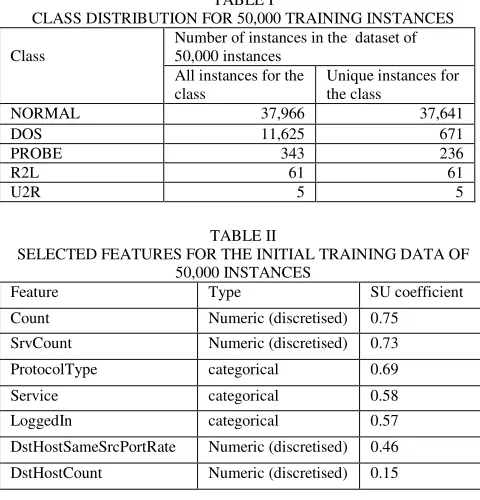
The initial Naïve Bayes model was constructed using the first 50,000 instances of the KDD Cup 1999 dataset. Table I shows the class distribution for these 50,000 instances. The initial set of predictive features was also selected based on these instances. Numeric features were each discretised into 10 intervals using equal-width binning [5], [17]. Table II provides a description of the features selected from the 50,000 instances using the SU coefficient. Cohen [18] has recommended that correlations with a magnitude less than 0.1 have no practical significance. For this reason, features with an SU coefficient less than 0.1 were considered to be irrelevant and were excluded from the classification process.

TABLE I

CLASS DISTRIBUTION FOR 50,000 TRAINING INSTANCES Number of instances in the dataset of 50,000 instances

Class

All instances for the

class Unique instances for the class NORMAL 37,966 37,641 DOS 11,625 671 PROBE 343 236

R2L 61 61

U2R 5 5

TABLE II

SELECTED FEATURES FOR THE INITIAL TRAINING DATA OF 50,000 INSTANCES

Feature Type SU coefficient Count Numeric (discretised) 0.75 SrvCount Numeric (discretised) 0.73 ProtocolType categorical 0.69 Service categorical 0.58 LoggedIn categorical 0.57 DstHostSameSrcPortRate Numeric (discretised) 0.46 DstHostCount Numeric (discretised) 0.15

It was stated in Section IIE that the m estimate of probability solves the problem of having cells with zero counts or vey small counts in a contingency table. For stream mining using Naïve Bayes classification this estimate may be needed for the computation of the likelihood terms (Pr(x_i|c_j)) since there is a high prevalence of zero counts in the contingency table cells. In fact, for the KDD Cup 1999 dataset, it was observed that for all (feature, class) contingency tables there is a very high occurrence of zero counts in the contingency tables for all time windows. Two

of the contingency tables are given in the appendix in order to illustrate this problem. Unfortunately, there are no clear guidelines in the literature on how to set the m value. Experiments were conducted to determine the appropriate m value, using the same 50,000 as a basis for Naïve Bayes classification. The same 50,000 instances were used for the construction of the contingency tables and for the testing of classification performance. Table III shows the classification results for these experiments. The accuracy and true positive rates (TPRATE%) on the classes are given in the table. The true positive rate for each class is computed as TPRATE = (number classified correctly / number in the test data). The m values of 0, L, 10L, 20L, and 30 were used for L probability estimation. The results of Table III indicate that for the classes with a large number of instances (NORMAL and DOS) changes in the m value do not affect the classification performance. However, for the classes with a very small number of instances (R2L and U2R), small values of m provide the best performance. Given these observations, the value of m = 0 was selected for the Naïve Bayes probability computations for the experiments.

TABLE III

CLASSIFICATION RESULTS FOR 50,000 TEST INSTANCES Naïve Bayes classification accuracy% and class TPRATE% for class:

m value

A

ll

cl

as

se

s

N

O

RM

A

L

D

O

S

PR

O

B

E

R

2L _U2R

0 97.4 99.5 90.5 96.8 90.2 80.0 L 97.2 99.4 90.5 94.8 88.5 0.0 10L 96.6 98.6 90.5 94.3 0.0 0.0 20L 96.4 98.4 90.5 91.8 0.0 0.0 30L 96.2 98.2 90.5 91.3 0.0 0.0

B. Stream mining experiments

Three alternative models were used for the stream mining experiments. The model MsA (s = 2,3,4,5) corresponds to the alternative of adding 1,000 new instances to the training dataset without removing any old instances. The model MsB corresponds to the alternative of adding 1,000 new instances and removing the 1,000 oldest instances. The model MsC corresponds to the alternative of adding 1,000 new instances and keeping only the newest 10,000 instances. Fig. 1 provides a representation of the sliding windows W2, W3, W4 and W5 for model creation and the time periods T2, T3, T4 and T5 for testing the model predictive accuracy. The testing periods T2,..,T5 are consecutive periods which respectively correspond to time periods when a batch of 1,000 new instances have arrived and have been classified by the models MsA, MsB and MsC which are created for the sliding windows W2, W3, W4 and W5.

continuous feature selection are shown in column 4. Testing period T2 appears to be a period of concept drift since the accuracy plummets to 3.3%. After T2 has passed, the accuracy results for testing periods T3, T4 and T5 indicate that in general the use of features selected at the beginning of each sliding window period results in either the same level of NB predictive accuracy as for period T3 or higher levels of predictive accuracy as for T4 and T5.

Fig. 1: Representation of models for the sliding window periods (Wi) and testing periods (Ti) for i = 2, 3, 4, 5.

TABLE IV

MODEL ACCURACY FOR TWO FEATURE SELECTION METHODS Testing

period (test

instances) Model

Accuracy % on fixed feature selection (7 features)

Number of features for continuous feature selection

Accuracy on continuous feature selection M2A 3.3 7 3.3 M2B 3.3 7 3.3 T2

(1000) _{M2C 3.3 21 3.3} M3A 97.2 7 97.2 M3B 97.2 7 97.2 T3

(1000) _{M3C 97.4 20 98.4} M4A 57.6 9 69.5 M4B 57.6 9 69.5 T4

(1000) _{M4C 55.2 17 55.1} M5A 43.3 9 91.0 M5B 43.3 9 91.0 T5

(1000) _{M5C 91.7 15 92.0}

A detailed analysis of the classification performance is provided in Tables V and VI. For each class, the number of instances present in the test data is given in column 1. The true positive rates (TPRATE%) for each class are given in columns 3 through 6. The U2R class did not appear in the part of the data stream that was used for the experiments, so it is not shown in the tables. The results of Tables V and VI indicate that the NORMAL class is generally very easy to predict correctly and both methods of feature selection provide high TPRATES for this class. The PROBE class is also generally easy to predict correctly. However, fixed feature selection provides higher predictive performance for time period T4. The DOS class is very difficult to predict for time periods T2 and T4. For period T2 there are no correct predictions for DOS by any of the models for both feature selection methods. For period T4 the models which use fixed feature selection fail to make any correct predictions for DOS while two of the models which use continuous

feature selection manage to achieve a TPRATE of 29.5% for the DOS class.

TABLE V

MODEL TPRATES FOR THE FIXED FEATURE SELECTION METHOD

Naïve Bayes classification performance for fixed feature selection

TPRATE% for class: Testing

period (class counts in test dataset)

Model

NORMAL DOS PROBE R2L M2A 100 0 0 M2B 100 0 0 T2

(NRM: 33 DOS: 965

R2L: 2 ) M2C 100 0 0 M3A 98.4 100 M3B 98.4 100 T3

(NRM: 539 PRB: 461 )

M3C 95.2 100 M4A 99.8 0 96.2 0 M4B 99.8 0 96.2 0 T4

(NRM: 552 DOS: 417 PRB: 26 R2L: 5 )

M4C 100 0 0 0 M5A 43.3

M5B 43.3 T5

(DOS: 1000)

M5C 91.7 TABLE VI

MODEL TPRATES FOR THE CONTINUOUS FEATURE SELECTION METHOD

Naïve Bayes classification performance for continuous feature selection

TPRATE% for class: Testing

period (class counts in test dataset)

Model

NORMAL DOS PROBE R2L

M2A 100 0 0 M2B 100 0 0 T2

(NRM: 33 DOS: 965

R2L: 2 ) M2C 100 0 0 M3A 94.8 100 M3B 94.8 100 T3

(NRM: 539

PRB: 461 ) _{M3C 97.0 100} M4A 99.9 29.5 80.8 0 M4B 99.9 29.5 80.8 0 T4

(NRM: 552 DOS: 417 PRB: 26 R2L: 5 )

M4C 100 0 0 0 M5A 91.0

M5B 91.0 T5

(DOS: 1000)

M5C 92.0

V. CONCLUSIONS

The main objective for the studies reported in this paper was to determine whether the use of continuous feature selection for the sliding window technique of stream mining based on Naïve Bayes classification leads to improved predictive performance. The experimental results reported in Section IV have indicated that for the dataset used in the experiments, continuous feature selection leads to improved predictive performance. It was pointed out in Section II that there is a need to employ fast methods of modeling for stream mining. A fast method of feature selection for Naïve Bayes stream mining has been presented in this paper. This method uses the same up-to-date data, stored in contingency Time

and instance arrival

Wi Ti

Training instances for model in window Wi:

MsA: 50,000 + (i-1)*1000

Test instances in test period Ti: 1,000

MsB: 50,000

tables, for both feature selection and Naïve Bayes classification.

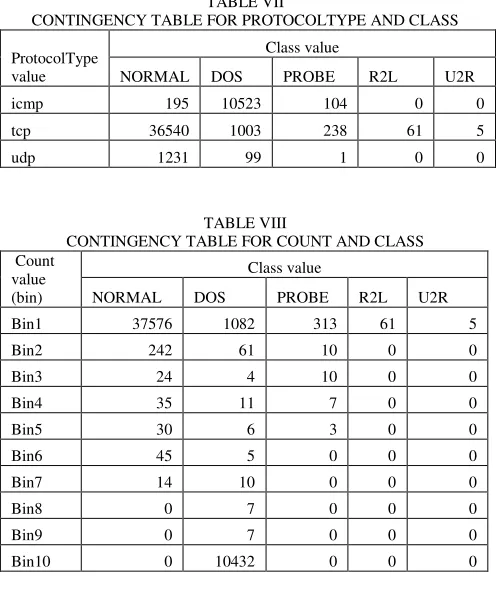
APPENDIX

Tables VII and VIII respectively show the feature-class contingency tables for the ProtocolType and Count features for the first 50,000 instances of the KDD Cup 1999 training dataset. Each numeric entry in a table cell shows the frequency of co-occurrence of one (feature-value, class- value) pair.

TABLE VII

CONTINGENCY TABLE FOR PROTOCOLTYPE AND CLASS Class value

ProtocolType

value NORMAL DOS PROBE R2L U2R icmp 195 10523 104 0 0 tcp 36540 1003 238 61 5 udp 1231 99 1 0 0

TABLE VIII

CONTINGENCY TABLE FOR COUNT AND CLASS Class value

Count value

(bin) NORMAL DOS PROBE R2L U2R Bin1 37576 1082 313 61 5 Bin2 242 61 10 0 0 Bin3 24 4 10 0 0 Bin4 35 11 7 0 0 Bin5 30 6 3 0 0 Bin6 45 5 0 0 0 Bin7 14 10 0 0 0 Bin8 0 7 0 0 0 Bin9 0 7 0 0 0 Bin10 0 10432 0 0 0

REFERENCES

[1] C.C. Aggarwal (ed), Data Streams: Models and Algorithms, Boston: Kluwer Academic Publishers, 2007.

[2] J. Gao, W. Fan and J. Han, “On appropriate assumptions to mine data streams: analysis and practice”, Proceedings of the Seventh IEEE International Conference on Data Mining (ICDM 2007), IEEE Computer Society, 2007.

[3] M.M. Masud, Q. Chen and J. Gao, “Classification and novel class detection of data streams in a dynamic feature space”, Proceedings of European Conference on Machine Learning and Practices in Knowledge Discovery from Databases (ECML/PKDD 2010), LNAI, 337-352, Springer-Verlag, 2010.

[4] J. Gao, W. Fan, J. Han and P.S. Yu, “A general framework for mining concept-drifting data streams with skewed distributions”, Proceedings of the SDM Conference, 2007.

[5] G. Hebrial, “Data stream management and mining”, In F. Fogelman-Soulié et al. (eds), Mining Massive Data Sets for Security, IOS Press, 2008.

[6] M.M. Gaber, A. Zaslavsky and S. Krishnaswamy, “Mining data streams: a review”, SIGMOD Record, vol. 34, no. 2, pp. 18- 26, 2005. [7] R. Munro and S.Chawla, “An integrated approach to mining data streams”, Technical Report TR-548, School of Information Technologies, University of Sydney, 2004.

[8] H. Liu and H. Motoda, Feature Selection for Knowledge Discovery and Data Mining, Boston: Kluwer Academic Publishers, 1998.

[9] R. Kohavi, “Scaling up the accuracy of Naïve Bayes classifiers: a decision tree hybrid”, Proceedings of the Conference on Knowledge Discovery from Databases (KDD 1996), pp 202-207, 1996.

[10] G.H. John, R. Kohavi and K. Pleger, “Irrelevant features and the subset selection problem”, In W.W. Cohen & H. Hirsh (eds), Proceedings of the 11th International Conference on Machine Learning, pp 121-129, 1994.

[11] G. Webb, J.R. Boughton and Z. Wang, “Not so Naïve Bayes: averaged one-dependence estimators”, Machine Learning, vol. 58, no. 1, pp. 5-24, 2005.

[12] A.P. White and W.Z. Liu, “Bias in information-based measures in decision tree induction”, Machine Learning, vol. 15, pp. 321-329, Boston: Kluwer Academic Pubications, 1994.

[13] T.M. Mitchell, Machine Learning, Burr Ridge, IL:WCB/McGraw Hill, 1997.

[14] B. Cestnik, “Estimating probabilities: a crucial task in machine learning”, Proceedings of the 9th European Conference on Artificial Intelligence , pp. 147-149, London: Pitman, 1990.

[15] S.D. Bay, D. Kibler, M.J. Pazzani and P. Smyth, “The UCI KDD archive of large data sets for data mining research and experimentation”, ACM SIGKDD, vol. 2, no. 2, pp. 81-85, 2000. [16] S.W. Shin and C.H. Lee, “Using Attack-Specific Feature Subsets for

Network Intrusion Detection”, Proceedings of the 19th Australian Conference on Artificial Intelligence. Hobart, Australia, 2006. [17] Y. Yang and G.I. Webb, “A comparative study of dicretization

methods for Naïve Bayes classifiers”, Proceedings of the Pacific Rim Knowledge Acquisition Workshop, PKAW 2002, pp. 159-173, 2002. [18] J. Cohen, Statistical Power Analysis for the Behavioural Sciences,