Double JPEG compression forensics based on a convolutional neural network

(1)

R E S E A R C H

Open Access

Double JPEG compression forensics based

on a convolutional neural network

Qing Wang

1,2

and Rong Zhang

1,2*

Abstract

Double JPEG compression detection has received considerable attention in blind image forensics. However, only few techniques can provide automatic localization. To address this challenge, this paper proposes a double JPEG

compression detection algorithm based on a convolutional neural network (CNN). The CNN is designed to classify histograms of discrete cosine transform (DCT) coefficients, which differ between single-compressed areas (tampered areas) and double-compressed areas (untampered areas). The localization result is obtained according to the

classification results. Experimental results show that the proposed algorithm performs well in double JPEG compression detection and forgery localization, especially when the first compression quality factor is higher than the second.

Keywords:Blind image forensics, Double JPEG compression, Convolutional neural network, Classification

1 Introduction

Generally, blind forensics techniques utilize statistical and geometrical features, interpolation effects, or feature inconsistencies to verify the authenticity of image/videos when no prior knowledge of the original sources is avail-able. Because JPEG compression may cover certain traces of digital tampering, many techniques are effective only on uncompressed images. However, most multi-media capture devices and post-processing software suites such as Photoshop, output images in the JPEG format, and most digital images on the internet are also JPEG images. Hence, developing blind forensics tech-niques that are robust to JPEG compression is vital. Tampering with JPEG images often involves recompres-sion, i.e., resaving the forged image in the JPEG format with a different compression quality factor after digital tampering, which may introduce evidence of double JPEG compression. Recently, many successful double JPEG compression detection algorithms have been pro-posed. Lukášand Fridrich [1] and Popescu and Farid [2] have performed some pioneering work. They analyzed the double quantization (DQ) effect before and after tampering and found that the discrete cosine transform (DCT) coefficient’s histograms for an image region that

has been quantized twice generally show a periodicity,

differing from the DCT coefficient’s histograms for a

single-quantized region. Chen and Hsu [3] identified periodic compression artifacts in DCT coefficients in ei-ther the spatial or Fourier domain, which can detect both block-aligned and nonaligned double JPEG com-pression. Fu et al. [4] and Li et al. [5] reported that DCT coefficients of single-compressed images generally follow

Benford’s law, whereas those of double-compressed

im-ages violate it. In [5], they detect double-compressed JPEG images by using mode-based first digit features combined with Fisher linear discriminant (FLD) analysis. Fridrich et al. [6] applied double JPEG compression in steganography. The feature they used is derived from the statistics of low-frequency DCT coefficients, and it is ef-fective not only for normal forged images but also for images processed using steganographic algorithms.

However, a commonality among all algorithms dis-cussed above is that they estimate only the compression history of an image, which cannot indicate exactly which region has been manipulated. In fact, the localization of tampered regions is a basic necessity for meaningful image forgery detection. Nevertheless, to the best of our knowledge, only few forensics algorithms can achieve it. Lin et al.’s algorithm [7] was the first to automatically lo-cate local tampered areas by analyzing the DQ effects

hidden among the DCT coefficient’s histograms. The

authors applied the Bayesian approach to estimate the * Correspondence:[email protected]

1_{Department of Electronic Engineering and Information Science, University of}

Science and Technology of China, Huangshan Road, Hefei, China 2_{Key Laboratory of Electromagnetic Space Information, Chinese Academy of}

Sciences, Huangshan Road, 230027 Hefei, China

(2)

probabilities of individual 8 × 8 block being untampered. In this way, the obtained block posterior probability map (BPPM) would show a visual difference between

tam-pered (single-compressed) regions and unchanged

(double-compressed) regions. To locate the tampered re-gions more accurately, Wang et al. [8] utilized the prior knowledge that a tampered region should be smooth and clustered and minimized a defined energy function using the graph cut algorithm to locate the tampered re-gions. Verdoliva et al. [9] explored a new feature-based technique using a conditional joint distribution of resid-uals for localization, which is computationally efficient and is not affected by the scene content. Bianchi et al. [10] proposed more reasonable probability models based on [7]. The algorithm computes a likelihood of each 8 × 8 block being doubly compressed, combined with a useful method of estimating the primary quantization QF1. This method exhibits a better performance than that proposed in [7]. Based on an improved statistical model, the method presented in [11] can detect either block-aligned or block-nonblock-aligned compressed tampered re-gions. Amerini et al. [12] localized the results of image splicing attacks based on the first digit features of DCT coefficients and employed a support vector machine (SVM) for classification. However, these methods function poorly when QF1 > QF2.

As it is well known, deep learning methods are able to learn features and perform classification automatically. Deep learning using convolutional neural networks (CNNs) has achieved considerable success in many fields, such as speech recognition, image classification or rec-ognition, document analysis, and scene categorization. For steganalysis, Qian et al. [13] and Pibre et al. [14] applied a CNN to learn features automatically and capture the complex dependencies that are useful for steganalysis, and the results are inspiring. Indeed, hierarchical feature learning using CNNs can learn specific feature representa-tion. We consider that CNNs with deep model can also be effective for blind image forensics.

In this paper, we propose to distinguish double JPEG compression forgeries and achieve localization by employ-ing a trainemploy-ing/testemploy-ing procedure usemploy-ing a CNN. To enhance

the effect of the CNN, we perform preprocessing on the DCT coefficients. The histograms of the DCT coefficients were extracted as the input, and then, a one-dimensional CNN is designed to learn features automatically from these histograms and perform classification. Finally, the tampered regions are located based on the classification results. The proposed technique is also compared with the schemes presented in [5, 6, 11] and the localization tech-nique proposed in [12].

The organization of the rest of the paper is as follows. In Section 2, we introduce some background regarding double JPEG compression. Then, we propose our CNN-based double JPEG compression detection and localization algorithm in Section 3. Experimental results and a per-formance analysis are presented in Section 4. Finally, we conclude in Section 5.

2 Background on double JPEG compression

Lukášand Fridrich [1] first identified the statistical prop-erties of double peaks that appear in DCT histograms as a result of double compression. Popescu and Farid [2] presented periodic artifacts in DCT histograms and ana-lyzed the DQ effect in detail, and Lin et al. [7] explored the use of the DQ effect for image forgery detection. In this section, we simply review the model of double JPEG compression. JPEG compression is an 8 × 8 block-based scheme. The DCT is applied to 8 × 8 blocks of the input image; then, the DCT coefficients are quantized, and a rounding function is applied to them. The quantized co-efficients are further encoded via entropy encoding. The quantization of the DCT coefficients is the main cause of information loss in the compressed image. The quantization table corresponds to each specific compres-sion quality factor (QF), which is an integer ranging from 0 to 100; a lower QF indicates that more informa-tion is lost.

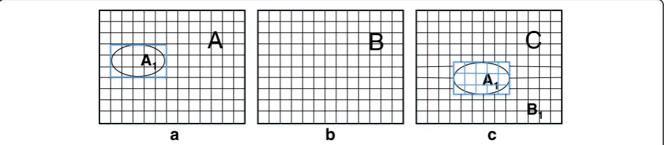
Double JPEG compression often occurs during digital manipulation. Here, we consider image splicing as an ex-ample; see Fig. 1:

(1) Cut and copy a regionA1 from imageA(of any format).

A

₁

B

C

A

1

B

1

a

b

c

(3)

(2) Decompress a JPEG image B, whose quality factor is QF1, and insertA1 intoB. LetB1 denote the unchanged background region ofB.

(3) Resave the new composite imageCin the JPEG format, with a JPEG quality factor QF2.

The new composite imageCconsists of two parts: the

inserted region A1 and the background region B1.B is

unquestionably doubly compressed, and we consider A1

to be singly compressed for the following reasons: (1) If

A is an image in a non-JPEG format, such as BMP or

TIFF, A1 is certainly singly compressed. (2) If A is a

JPEG image, then the DCT grids of A1 may not match

those of B or B1, and thus, this region will violate the

rules of double compression. Hence, the new image C

will exhibit a mixture of two characteristics:A1 is singly

compressed, and B1 is doubly compressed. There is a

small probability (1/64) that the tampered blocks will be exactly aligned with the unchanged blocks; however, this probability is small enough to be ignored.

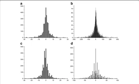
Double-quantized DCT coefficient histograms have certain unique properties. Figure 2 shows several exam-ples: Fig. 2a, b shows the DCT coefficient histograms for a single-compressed JPEG image at the (0,1) position in zigzag order for quality factors of QF1 = 60 and

QF1 = 90, respectively, and Fig. 2c, d shows the DCT coefficient histograms for the same image after double compression with QF1 = 90, QF2 = 60 and with QF1 = 60, QF2 = 90, respectively. We observe that the histograms after single compression at each frequency approximately follow a generalized Gaussian distribution, whereas double JPEG compression changes this distribution: when QF2 > QF1, the histogram after double compression exhibits periodically missing values, whereas when QF2 < QF1, the histogram exhibits a periodic pattern of peaks and valleys. In both cases, the histogram can be regarded as exhibiting periodic peaks and valleys.

We use the histograms of DCT coefficients as the in-put to the CNN that is designed to automatically learn the features of these histograms and perform classifica-tion for single and double JPEG compression.

3 Proposed model

In Section 2, we analyzed how recompression affects the distribution of the DCT coefficients. In this section, we exploit this knowledge to define a set of significant fea-tures that should be insensitive to recompression and design a one-dimensional CNN to learn and classify these features.

Fig. 2DCT coefficient histograms corresponding to the (0,1) position.a,bDCT coefficient histograms of a single-compressed image withaQF1 = 60 andbQF1 = 90.c,dDCT coefficient histograms of the same double-compressed image withcQF1 = 90, QF2 = 60, and

(4)

Preprocessing for a given JPEG image, we first extract its quantized DCT coefficients and the last quality factor from the JPEG header. In our experiment, we use only the Y component of color images. Then, we construct a histogram for each DCT frequency.

In this paper, we consider only the AC coefficients. We strongly believe that our method could also work for the DC term, as well, whereas the distribution of the DC coef-ficient’s histogram is different from that of the AC ones, which may bring difficulty of feature design. Therefore, only AC coefficients are taken into account. Besides, it is difficult to operate if the whole histograms are fed to the CNN classifier directly, for the following reasons: (1) The input feature dimensions of the CNN must be consistent, while histograms always have variable sizes. (2) An exces-sively high computational cost for training may be in-curred. To reduce the dimensionality of the feature vector without losing significant information, a specified interval near the peak of each histogram (which may contain most of the significant information) is chosen to represent the whole histogram. We use the following method to extract feature sets at the low frequencies: first, the 2nd–10th co-efficients arranged in zigzag order are chosen to construct the feature sets, and only the values corresponding to the positions at {−5,−4,...4, 5} are considered as useful fea-tures. The details are illustrated below:

Let B denote a block with a size of W×W, and let

hi(u) denote the histogram of DCT coefficients with the valueu at the ith frequency in zigzag order in B. Then, the feature set consists of the following values:

XB¼ fhið Þ;−5 hið Þ;−4 hið Þ;−3 hið Þ;−2 hið Þ;−1 hið Þ;0 hið Þ;1 hið Þ;2 hið Þ;3 hið Þ;4 hið Þ5 ji∈2;3…;9;10g

In this way, we obtain a 9 × 11 feature for each block. In Section 4.5, we discuss the detection accuracy using different feature vector sizes.

3.1 The CNN architecture

A CNN relies on three concepts: local receptive fields, shared weights, and spatial subsampling [15]. In each convolutional layer, the output feature map generally represents convolution with multiple inputs, which can capture local dependencies among neighboring ele-ments. Each convolutional connection is followed by a pooling layer that performs subsampling in the form of local maximization or averaging; such subsampling can reduce the dimensionality of the feature map and, fur-thermore, the sensitivity of the output. After these alter-nating convolutional and pooling layers, the output feature maps pass through several full connections and then are fed into the final classification layer. This classi-fication layer uses a softmax connection to calculate the distribution of all classes.

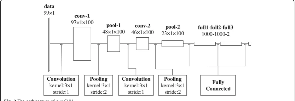
The architecture of our network is shown in Fig. 3. It contains two convolutional connections followed by two pooling connections and three full connections. The size of the input data is 9 × 11, and the output is a distribu-tion of two classes.

For the convolutional connections, we set the kernel size (m×n) to 3 × 1, the number of kernels (k) to 100, and the stride (s) to 1. Here, we consider the first convo-lutional layer as an example: the size of the input data is 99 × 1, and the first convolutional layer convolves these data with 100 3 × 1 kernels, with a stride (step size) of 1. The size of the output is 97 × 1 × 100, which means that the number of feature maps is 100 and the output fea-ture maps have dimensions of“97 × 1”.

For the pooling connections, we set the pooling size (m×n) to 3 × 1, and the pooling stride (s) to 2, and we select max pooling as the pooling function. We observe that such overlapping pooling prevent overfitting during training.

Each full connection has 1000 neurons, and the output of the last one is sent to a two-way softmax connection, which produces the probability that each sample should

Convolution kernel:3×1

stride:1 data 99×1

conv-2 46×1×100

pool-2 23×1×100

full1-full2-full3 1000-1000-2

Pooling kernel:3×1

stride:2

Convolution kernel:3×1

stride:1

Pooling kernel:3×1

stride:2

Fully Connected conv-1

97×1×100

pool-1 48×1×100

(5)

be classified into each class. In the context of blind image forgery detection, there are only two classes: authentic (doubly compressed) and forged (singly compressed).

In our network, rectified linear units (ReLUs), with an activation function of f(x) = max(0,x), are used for each connection. In [16], it was proven that deep learning networks with ReLUs converge several times faster than tanh and also exert considerable influence on the training performance for a large database. In both fully

connected layers, the recently introduced “dropout”

technique [17] is used. The key idea is to randomly drop units from the neural network during training, which provides a means of efficiently combining different net-work architectures. With the dropout technique, overfit-ting can be effectively alleviated.

The choice of the CNN structure and the selection of the model parameters will be discussed in Section 4.5.

3.2 Locating tampered regions

To achieve localization, the image of interest, I, with a resolution of M×N, is divided into overlapping blocks with a dimension ofW×W, and an overlapping stride of 8 pixels, the size of the blocks on which DCT is per-formed during JPEG compression. Thus, we obtain a total of () (⌈(M−W)/8⌉+ 1) × (⌈(N−W)/8⌉+ 1) blocks from one image. For each block, a 9 × 11 feature vector, as described in detail in Section 3.1, is computed and fed to the designed CNN. The output of the CNN is a prob-ability pair [a,b], where a is the probability that the block is singly compressed andb is the probability that the block is doubly compressed. To achieve localization, we use the a values to obtain a classification result for each block, and the center 8 × 8 part of each block will

be set to the same value equal toa. Thus, a detection re-sult map with the same resolution of the original inter-ested image and the tampering mask is obtained (the (W−8)/2 pixels at the edge of the image will be padded to zeros). Higher values in this map indicate higher probabilities that the corresponding blocks are singly compressed, which are shown visually as whiter regions in the result map.

4 Experimental results and performance analysis

In this section, we test the ability of our algorithm to de-tect double JPEG compression and composite JPEG im-ages. To demonstrate the superiority of our method, we first compare the accuracy of double JPEG compression detection for different block sizes with the method proposed in [5], which detects double-compressed JPEG images by using mode-based first digit features, and the method proposed in [6], which uses the statistics of low-frequency DCT coefficients. For composite JPEG image detection, we compare our localization results with the method proposed in [11], which achieves localization based on the DQ effects combined with Bayes’s theorem, and also with the technique proposed in [12] based on Benford’s law using SVM.

4.1 The database

For the experimental validation, we built an image database consisting of training, validation and testing datasets.

(1) Training and validation datasets. The uncompressed images in UCID [18], consisting of 1338 TIFF images with a resolution of 512 × 384 (or 384 × 512),

60 70 80 90 100

0.65 0.70 0.75 0.80 0.85 0.90 0.95 1.00

accuracy

QF₂

64x64 128x128 256x256 512x512 1024x1024

(6)

were chosen for training and validation purposes. We randomly selected 800 images to serve as training data for the neural network and 200 images to serve as validation data. To create single-compressed images, these images were single-compressed with QF2∈{60, 65,...90.95}, respectively. To create double-compressed images, these TIFF images were compressed with QF1∈{60, 70, 80, 90, 95}, respectively, followed by recompression with QF2∈{60, 65,...90, 95}. For both training and validation process, we performed overlapping cropping to crop them to dimensions of 64 × 64

with a stride of 32 pixels, leading to a total amount of 132,000 elements for each positive set and negative set.

(2) Testing dataset. For better experimental validation of the proposed work, we applied two databases with different resolutions which are commonly used in image forensics literature for testing process. The low-resolution repository is from the rest images in UCID with a resolution of 512 × 384, and the high-resolution repository is from the Dresden Image Database [19], which contains 736 uncompressed RAW images of 3039 × 2014 pixels using a Nikon

60 70 80 90 100

0.65 0.70 0.75 0.80 0.85 0.90 0.95 1.00

accuracy

QF₂

64x64

128x128

256x256

512x512

1024x1024

Fig. 5Accuracy of [5] for different quality factors QF2 and different image sizes

60 70 80 90 100

0.40 0.45 0.50 0.55 0.60 0.65 0.70 0.75 0.80 0.85 0.90 0.95 1.00

accuracy

QF₂

64x64

128x128

256x256

512x512

1024x1024

(7)

D70 camera and 752 uncompressed RAW images of 3900 × 2616 pixels acquired with a Nikon D200 camera. To obtain composite tampered JPEG images, 100 images were randomly selected from both of the two databases, compressed with quality factors of QF1∈{60, 70, 80, 90, 95}, respectively, and then been spliced with a rectangular block randomly selected from either JPEG images or non-JPEG images using the Photoshop software. The rectangular block is randomly put on the background image. Finally, each composite image was compressed with quality factors of QF2∈{60, 65,...90, 95}, respectively. The authentic image sets consist of images compressed only once with QF2∈{60, 65,...90, 95}. Furthermore, all the tampered regions in both of the two databases cover approximately the 2 % of the total surface, namely a size of 384 × 384 in high-resolution datasets and a size of 64 × 64 in low-resolution datasets. It is worth mentioning that each image in our database is associated with a tampering mask, providing a convenient shortcut for validating the performance of the algorithm. Both of the two databases are accessible online [1].

It should be noted that we have to construct a classi-fier for each secondary quality factor QF2 because of the unknown primary quality factor QF1. Thus, we obtained eight different two-class classifiers corresponding to each value of QF2 (QF2∈{60, 65,...90, 95}) in our experiment. For most machine learning techniques employing a training/testing procedure, there are difficulties in cor-rectly classifying images as double-compressed when

QF1 is different from the ones used in the training set. As no priori information on the previous history is generally available to the analyst in actual forensics situation, for an actual training/testing procedure, it is best to make all the possible QF1 (range from 50 to 100) be traversed in the training sets to make the classifiers work well. In this paper, we only select some representa-tive QF1 and QF2 for experiment to show the effecrepresenta-tive- effective-ness of the CNN classifiers.

Fig. 7Detection results.a,eImages manipulated with Photoshop compressed with QF1 = 70, QF2 = 90 and QF1 = 60, QF2 = 95.b,fThe original authentic images corresponding toaande.c,gThe classification result maps obtained using the proposed algorithm.d,hThe tampering masks

Table 1AUC values achieved on the Dresden Image Database by the proposed algorithm and the algorithms presented in [11] and [12]

QF2 60 65 70 75 80 85 90 95

QF1

60 Proposed 0.68 0.88 0.95 0.96 0.99 0.99 1.00 0.99

Bayesian approach 0.50 0.83 0.97 0.99 0.99 0.99 0.99 0.99

SVM 0.50 0.81 0.90 0.75 0.74 0.74 0.94 0.96

70 Proposed 0.95 0.86 0.67 0.85 1.00 1.00 1.00 0.99

SVM 0.72 0.71 0.68 0.70 0.75 0.75 0.97 0.98

80 Proposed 0.98 0.94 0.99 0.94 0.44 0.99 1.00 0.99

SVM 0.50 0.71 0.88 0.81 0.40 0.87 0.85 0.97

90 Proposed 0.89 0.78 0.91 0.81 0.97 0.97 0.45 1.00

SVM 0.54 0.65 0.71 0.64 0.71 0.72 0.65 0.99

95 Proposed 0.71 0.66 0.63 0.57 0.51 0.67 0.93 0.46

(8)

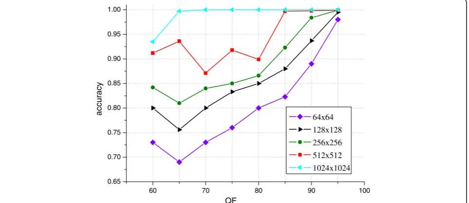
4.2 Detecting double JPEG compression

For this experiment, we used only the pure doubly and

singly JPEG compressed images from our

high-resolution datasets. We performed the experiment for five image sizes: W×W= 64 × 64; 128 × 128; 256 × 256; 512 × 512, and 1024 × 1024. Figure 4 shows the accuracy of our proposed CNN for the different quality factors QF2 averaged over all QF1 and for the different image sizes. Figures 5 and 6 show the results of [5] and [6]

for comparison. It is obvious that our classifier ex-hibits a better performance in most cases especially when QF2 < 90. Moreover, a larger training image size leads to higher accuracy for all of the detectors. For [6], the classifiers even do not work when the image size is as small as 64 × 64, while our CNN approach can work well in this situation.

Meanwhile, we also compared our proposed architec-ture to other machine learning techniques in the same experimental settings: The designed 9 × 11 feature vec-tors were fed into SVM classifiers and Fisher linear dis-criminant (FLD) analysis which was mentioned in [5] to perform classification. But it turns out to be a failure, and neither SVM classifiers nor FLD classifiers can dif-ferentiate the designed features obtained from single-compressed images and double-single-compressed images, which indicates that it is hard to perform classification on these designed features using these traditional ma-chine learning techniques. The reason we consider is that traditional machine learning techniques are limited in their ability to process data in their raw form.

They usually require carefully designed feature extrac-tors to transform the raw data into a suitable representa-tion, from which the machine can classify patterns in its input. Deep learning methods are representation learn-ing methods [20], which allow a machine to be fed with raw data and to automatically learn the representations needed for classification. Indeed, hierarchical feature learning using the CNN deep models can learn specific feature representation automatically, which is difficult for most traditional machine learning techniques. For double-compression detection in blind forensics, the histograms of doubly compressed images contain DQ

Table 2AUC values achieved on the UCID database by the proposed algorithm and the algorithms presented in [11] and [12]

QF2 60 65 70 75 80 85 90 95

QF1

60 Proposed 0.64 0.93 0.95 0.97 0.98 0.98 0.94 0.91

SVM 0.43 0.73 0.84 0.80 0.81 0.78 0.78 0.88

70 Proposed 0.88 0.87 0.52 0.79 0.96 0.96 0.98 0.94

SVM 0.70 0.66 0.57 0.75 0.80 0.80 0.84 0.85

80 Proposed 0.93 0.89 0.89 0.88 0.52 0.97 0.98 0.96

SVM 0.50 0.59 0.74 0.74 0.44 0.74 0.73 0.89

90 Proposed 0.74 0.81 0.73 0.57 0.79 0.82 0.48 0.95

SVM 0.45 0.44 0.54 0.60 0.74 0.73 0.52 0.91

95 Proposed 0.67 0.73 0.66 0.66 0.65 0.70 0.71 0.50

SVM 0.56 0.57 0.61 0.56 0.55 0.48 0.67 0.54

55 60 65 70 75 80 85 90 95 100

0.54 0.60 0.66 0.72 0.78 0.84 0.90 0.96

AUC

QF₂

Proposed Method Reference Method [10] Reference Method [11]

(9)

55 60 65 70 75 80 85 90 95 100 0.54

0.60 0.66 0.72 0.78 0.84 0.90 0.96

AUC

QF₂

Proposed Method Reference Method [10] Reference Method [11]

Fig. 9AUC comparison of the proposed method, the method of [11], and the method of [12] on the UCID database

(10)

effects which are quite different from the singly ones, and our proposed feature is the specified interval of these histograms. The traditional machine learning tech-niques can hardly learn these features if the histograms (raw data) are used directly for classification without any handcrafted feature extraction; however, the designed CNN can achieve representation learning automatically, which can easily capture the proposed signal that is im-portant for double JPEG compression detection. This would give insights on the actual benefits of the CNN approach.

4.3 Detecting composite JPEG images

In this experiment, we detected composite JPEG images. There is one thing worth to mention: it is a trade-off be-tween the need for sufficient statistics and the precision of manipulation detection. We tested many block sizes and ultimately chose to setWto 64.

Figure 7 shows several successful detection results of our algorithm. Figure 7a, e is tampered through a copy-paste operation using Photoshop. The second column shows the original images, the third column shows the classification result maps obtained using our proposed algorithm, and the rightmost column shows the masks used for comparison. It is clear that the classification result maps generally locate the tampered regions cor-rectly. Additional results, compared with those ob-tained using the methods of [11] and [12], are shown in Figs. 10 and 11 for different combinations of quality factors.

4.4 Performance analysis

In [11], the author introduced a method of measuring the performance of a forgery detector based on the area under the receiver operating characteristic (ROC) curve (AUC). The ROC curve is obtained from the false alarm

Fig. 11Detection results.aTampered images coming from the Dresden Image Database compressed with QF1 = 70, QF2 = 60 and QF1 = 80, QF2 = 70 (two at the top) and from the UCID database compressed with the same quality factors (two at the bottom).bThe classification result maps obtained using the proposed algorithm.cThe results of the method proposed in [11].dThe results of the method proposed in [12].eThe tampering masks

Table 3The accuracy of double JPEG compression detection using different numbers of connections

QF2/kernel size 1 conv 2 convs 3 convs

60 0.718 0.728 0.701

80 0.788 0.796 0.781

Table 4The accuracy of double JPEG compression detection using different kernel sizes

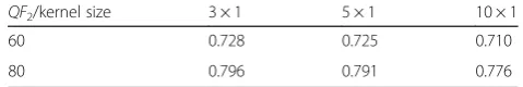
QF2/kernel size 3 × 1 5 × 1 10 × 1

60 0.728 0.725 0.710

(11)

probability Pf and the correct detection probability Pc, which are given byPf=Na/(Ni−Nt) andPc= 1−Nb/Nt

where Na is the number of blocks identified as forged

that have not actually been tampered with, Nb is the

number of blocks that have been tampered with but not

identified as forged, Ni is the number of blocks in the

entire image, and Nt is the total number of tampered

blocks. The area under the ROC curve is the AUC value, which is a number between 0 and 1, and a larger AUC value indicates better detector performance.

Table 1 shows the AUC values achieved on the Dresden Image Database (high-resolution) using our proposed method. For comparison, the AUC values for the methods proposed in [11] (Bayesian approach) and [12] (SVM) are also shown in Table 1. Table 2 shows the AUC values achieved on the UCID database (low-reso-lution) of all the three methods. The best results in each case are highlighted in italics (if all algorithms perform the same in a given case, none is highlighted). It is evi-dent that our method outperforms those of [11] and [12], especially for lower QF2 values: when QF2 > QF1, all methods have high AUC values of nearly 0.99, whereas when QF2 < QF1, our method has a better performance.

Figures 8 and 9 show the AUC comparisons averaged over all QF1 on both of the two datasets. It is important to note that we did not consider the case of QF2 = QF1 because double JPEG compression is generally defined

as QF2≠QF1 (Tables 1 and 2 also illustrate that it is

very difficult for either method to detect tampering when QF2 = QF1). It can be appreciated that our method per-forms much better than those of [11] and [12], especially when QF2 < QF1, for which our method achieves AUC values of nearly 0.86 on both high-resolution datasets and nearly 0.84 on low-resolution datasets.

We also present several further example results of detection obtained from both the high-resolution and low-resolution datasets, for our method compared with the methods of [11] and [12]. Figure 10 shows detection results corresponding to the case of QF2 > QF1, and Fig. 11 shows results corresponding to the case of QF2 < QF1. When QF2 > QF1, all methods clearly lo-cate the tampered regions. When QF2 < QF1, the results of the method presented in [11] and [12] contain large false alarm areas and the locations of the tampered re-gions are not as clearly visible, whereas our method performs better.

The computation complexity of the CNN is huge. The long learning times are due to the fact that the back-propagation process during the training of network has to be scanned many times until convergence, and these operations have to be done on a big database. Those computations can be accelerated through the use of GPU, and our experiments of the CNN are performed on a NVIDIA GTX 960 GPU. It takes 12 min to train an epoch and 60 min for the results to converge.

4.5 Selection of model parameters

We tested many CNN architectures. In this section, we present several experiments designed to reveal the accuracy of double JPEG compression detection using different model parameters and different CNN archi-tectures. (Note that we performed these tests only for QF2 = 60 and QF2 = 80.)

Tables 3, 4, and 5 present the accuracy of double JPEG compression detection achieved using different network connections, kernel sizes, and numbers of kernels. We can make the following observations: in terms of the network connections, an architecture with two sets of convolutional layers followed by pooling layers performs best. Generally, CNNs with more convolutional connec-tions deliver better results. Nonetheless, the deeper the CNN architecture is, the more information of high-layer semantic loses, probably due to the impact of the sub-sampling step such as pooling and convolution. There-fore, we use two convolutional layers in this paper; in terms of the kernel size, the results for a 3 × 1 kernel size are nearly identical to those for a 5 × 1 kernel size. In this paper, we set the kernel size to 3 × 1, and in terms of the number of kernels, a CNN with more kernels yields better results. However, there is a trade-off be-tween the precision of manipulation detection and the time cost. The use of more kernels requires more time for training: when 384 kernels are used, nearly 2 h is needed for training, whereas only 1 h is required when using 100 kernels. Therefore, we set the number of ker-nels to 100. Table 6 shows the relationship between the

Table 5The accuracy of double JPEG compression detection using different numbers of kernels

QF2/number of kernels

40 100 384

60 0.716 (51 min) 0.728 (60 min) 0.730 (120 min)

80 0.793 (52 min) 0.796 (60 min) 0.796 (120 min)

Table 6The accuracy of double JPEG compression detection using different training set sizes

QF2/total number of blocks

33,000 66,000 132,000 264,000 396,000

60 0.500 0.695 0.702 0.728 0.729

80 0.500 0.773 0.780 0.791 0.791

Table 7The accuracy of double JPEG compression detection using different feature dimensions

QF2/feature dimensions

7[₋3,3] 11[₋5,5] 21[₋10,10]

60 0.710 0.728 0.722

(12)

size of the training set (total number of blocks) and the performance of the classifier. The results show that fewer training images result in worse performance of the CNN. Moreover, when the number of training images is only one eighth of our recommended value, the CNN does not function at all. Whereas when the number of training images is 1.5 times with respect to the recom-mended value, the accuracy remains nearly unchanged. Table 7 shows the accuracy achieved using different feature vector sizes. In this paper, we used only the histogram values in the range of [−5, 5].

5 Conclusions

In this paper, a novel forensics methodology for detect-ing and localizdetect-ing double JPEG compression in images is proposed. We propose to identify and locate double JPEG compression forgeries using DCT coefficient’s his-tograms combined with a CNN deep model. Our method works well on small blocks, achieves localization automatically, and has a better performance especially when QF2 < QF1.

Although our proposed method produces encouraging results, it has some limitations: (1) the computational complexity of the CNN is considerably high, thus gener-ating a trade-off between the localization accuracy cap-ability and the computational effort required; (2) this method only constructs classifiers for different QF2, which will lead to lower detection accuracy due to the fact that the nature of the DCT coefficient histogram is quite different for different QF1. Further efforts are still needed: we consider that a CNN can be used to estimate QF1, and our future work will focus on the automatic estimation of QF1.

Acknowledgements

This work is supported by the National Nature Science Foundation of China under Grant No.61331020.

Authors_’contributions

QW and RZ carried out the main research of this work. QW performed the experiments. RZ conceived of the study, participated in its design and coordination, and helped draft the manuscript. All authors read and approved the final manuscript.

Competing interests

The authors declare that they have no competing interests.

Received: 22 January 2016 Accepted: 27 September 2016

References

1. J Lukáš, J Fridrich, Estimation of primary quantization matrix in double compressed JPEG images, inProc. Digital Forensic Research Workshop, 2003, pp. 5_–8

2. Popescu A C, Farid H. Statistical tools for digital forensics. International Workshop on Information Hiding. (Springer, Berlin Heidelberg 2004),pp. 128-47. 3. YL Chen, CT Hsu, Detecting recompression of JPEG images via periodicity

analysis of compression artifacts for tampering detection. IEEE Transactions on Information Forensics and Security6(2), 396–406 (2011)

4. Fu D, Shi Y Q, Su W. A generalized Benford's law for JPEG coefficients and its applications in image forensics.Electronic Imaging 2007. International Society for Optics and Photonics. 65051L-65051L-11(2007)

5. B Li, YQ Shi, J Huang, Detecting doubly compressed JPEG images by using mode based first digit features, in2008 IEEE 10th Workshop on Multimedia Signal Processing, 2008, pp. 730_–735

6. J Fridrich et al., Detection of double-compression in JPEG images for applications in steganography. IEEE Transactions on information forensics and security3(2), 247–258 (2008)

7. Z Lin, J He, X Tang, CK Tang, Fast, automatic and fine-grained tampered JPEG image detection via DCT coefficient analysis. Pattern Recognition

42(11), 2492–2501 (2009)

8. W Wang, J Dong, T Tan, Exploring DCT coefficient quantization effects for local tampering detection. IEEE Transactions on Information Forensics and Security9(10), 1653–1666 (2014)

9. Verdoliva L, Cozzolino D, Poggi G. A feature-based approach for image tampering detection and localization. 2014 IEEE International Workshop on Information Forensics and Security (WIFS). IEEE. 149-54(2014)

10. Bianchi T, De Rosa A, Piva A. Improved DCT coefficient analysis for forgery localization in JPEG images. 2011 IEEE International Conference on Acoustics, Speech and Signal Processing (ICASSP). IEEE. 2444-7(2011) 11. T Bianchi, A Piva, Image forgery localization via block-grained analysis of

JPEG artifacts. IEEE Transactions on Information Forensics and Security

7(3), 1003–1017 (2012)

12. Amerini I, Becarelli R, Caldelli R, et al. Splicing forgeries localization through the use of first digit features. 2014 IEEE International Workshop on Information Forensics and Security (WIFS). IEEE. 143-48(2014) 13. Qian Y, Dong J, Wang W, et al. Deep learning for steganalysis via

convolutional neural networks. SPIE/IS&T Electronic Imaging. International Society for Optics and Photonics. 94090J-94090J-10(2015)

14. L Pibre, P Jerome, D Ienco, M Chaumont,Deep learning for steganalysis is better than a rich model with an ensemble classifier, and is natively robust to the cover source-mismatch, 2015. arXiv preprint arXiv:1511.04855 15. Y Lecun, B Boser, JS Denker, D Henderson, RE Howard, W Hubbard, LD

Jackel, Backpropagation applied to handwritten zip code recognition. Neural Computation1(4), 541–551 (1989)

16. A Krizhevsky, I Sutskever, GE Hinton, ImageNet classification with deep convolutional neural networks, inAdvances in Neural Information Processing Systems, 2012, pp. 1097–1105

17. GE Hinton, N Srivastava, A Krizhevsky, I Sutskever, RR Salakhutdinov, Improving neural networks by preventing co-adaptation of feature detectors. ResearchGate3(4), 212_–223 (2012)

18. Schaefer G, Stich M. UCID: an uncompressed color image database. Electronic Imaging 2004. International Society for Optics and Photonics. 472-80(2003)

19. T Gloe, R Böhme Re, The Dresden Image Database for benchmarking digital image forensics. Journal of Digital Forensic Practice3(2-4), 150–159 (2010) 20. Y LeCun, Y Bengio, G Hinton, Deep learning. Nature521(7553), 436–444 (2015)