Ph.D. program in Computer Engineering
XXVII Cycle - 2015
Computing on Evolving Social Networks
Ph.D. program in Computer Engineering
XXVII Cycle - 2015
Francesco Ficarola
Computing on Evolving Social Networks
Thesis Committee
Prof. Andrea Vitaletti (Advisor) Prof. Luca Iocchi (Co-Advisor)
Reviewers
Prof. Giancarlo Ruffo Prof. Mirco Musolesi Dr. Emiliano Miluzzo
Dipartimento di Ingegneria Informatica, Automatica, Gestionale Sapienza Università di Roma
Via Ariosto 25, 00185 Roma, Italy e-mail: [email protected]
First and foremost I offer my honestest gratitude to my supervisor, Prof. Andrea Vitaletti, who introduced me to the wonderful world of research and inspired me throughout my thesis with his precious advice and inventiveness. I am also immensely thankful to Prof. Luca Becchetti and Prof. Aris Anagnostopoulos, two fantastic researchers. Along with Andrea, Luca and Aris have offered me a lot of their time, knowledge and friendship (as well as a lot of coffees). Moreover, I want to thank Prof. Alberto Marchetti-Spaccamela for supporting me over and over again.
My authentic gratitude goes to my friends Stefano Puglia and Luigi Teodonio, who spent their time in reading my thesis and giving me priceless suggestions. I wish to thank also all other friends for their constant moral support.
I am endless grateful to my mother and my father, who have made possible my dream.
Finally, I want to heartily thank Michela, my better half, who has followed me to the ends of the earth.
Over the past decade, participation in social networking services has seen an exponential growth, so that nowadays most individuals are “virtually” con-nected to others anywhere in the world. Consistently, analysis of human social behavior has gained momentum in the computer science research community. Several well-known phenomena in the social sciences have been revisited in a computer science perspective, with a new focus on phenomena of emerging behavior, information diffusion, opinion formation and collective intelligence. Furthermore, the recent past has witnessed a growing interest in the dynamics of these phenomena and that of the underlying social structures.
This thesis investigates a number of aspects related to the study of evolving social networks and the collective phenomena they mediate. We have mainly pursued three research directions.
The first line of research is in a sense functional to the other two and con-cerns the collection of data tracking the evolution of human interactions in the physical space and the extraction of (time) evolving networks describing these interactions. A number of available datasets describing different kinds of social networks are available on line, but few involve physical proximity of humans in real life scenarios. During our research activity, we have de-ployed several social experiments tracking face-to-face human interactions in the physical space. The collected datasets have been used to analyze network properties and to investigate social phenomena, as further described below.
A second line of research investigates the impact of dynamics on the an-alytical tools used to extract knowledge from social networks. This is clearly a vast area in which research in many cases is in its early stages. We have focused on centrality, a fundamental notion in the analysis and characteriza-tion of social network structure and key to a number of Web applicacharacteriza-tions and services. While many social networks of interest (resulting from “virtual” or “physical” activity) are highly dynamic, many Web information retrieval al-gorithms were originally designed with static networks in mind. In this thesis, we design and analyze decentralized algorithms for computing and maintain-ing centrality scores over time evolvmaintain-ing networks. These algorithms refer to notions of centrality which are explicitly conceived for evolving settings and
portant, yet not completely understood phenomenon of collective intelligence, whereby a group typically exhibits higher predictive accuracy than its single members and often experts. Phenomena of collective intelligence involve ex-change and processing of information among individuals sharing some common social structure. In many cases of interest, this structure is suitably described by an evolving social network. Studying the interplay between the evolution of the underlying social structure and the computational properties of the re-sulting process is an interesting and challenging task. We have focused on the quantitative analysis of this aspect, in particular the effect of the network on the accuracy of prediction. To provide a mathematical characterization, we have revisited and modified a number of models of opinion formation and dif-fusion originally proposed in the social sciences. Experimental analysis using data collected from some of the social experiments we conducted allowed to test soundness of the proposed models. While many of these models seem to capture important aspects of the process of opinion formation in (physical) social networks, one variant we propose achieves higher predictive accuracy and is also robust to the presence of outliers.
Introduction 1
I Evolving Social Networks 9
1 Evolving Networks 11
1.1 Social networks in the “static” case . . . 12
1.1.1 Representation and measurement of networks . . . 15
1.2 Social networks in dynamic contexts . . . 29
1.2.1 Representing and measuring evolving networks . . . 32
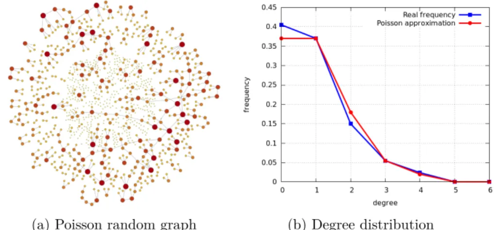
1.3 Random graph generative models . . . 38
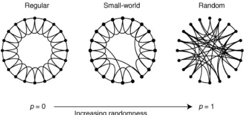
1.3.1 Erdős-Rényi model . . . 38 1.3.2 Wattz-Strogatz model . . . 39 1.3.3 Kleinberg model . . . 41 1.3.4 Barabási-Albert model . . . 42 1.4 Concluding remarks . . . 43 2 F2F Social Networks 45 2.1 Background on MAC protocols . . . 46
2.2 F2F social networks . . . 49
2.2.1 Technologies . . . 50
2.2.2 Applications . . . 52
2.3 Capture F2F interactions in real-world social scenarios . . . 53
2.4 Experiments and evaluation of the protocols . . . 56
2.4.1 Preliminary experiments . . . 56
2.4.2 Real-world social experiments . . . 58
2.4.3 Simulation on larger and denser graphs . . . 69
2.5 Concluding Remarks . . . 71
3 Decentralized Computation of Centrality Scores: the case of
PageRank 75
3.1 Related work . . . 77
3.2 Preliminaries . . . 79
3.2.1 Recap on evolving networks . . . 79
3.2.2 PageRank . . . 81
3.3 Defining Pagerank on evolving networks . . . 83
3.3.1 An experimental outlook . . . 83
3.3.2 PageRank of the expected network . . . 87
3.4 Fully decentralized Pagerank algorithms . . . 89
3.4.1 Analysis ofFDSAMPLEon homogeneous networks . . . . 90
3.4.2 Discussion . . . 96
3.4.3 Addressing non homogeneous networks . . . 98
3.5 Experimental analysis . . . 100
3.5.1 Evolving networks datasets . . . 101
3.5.2 Experiments on synthetic networks . . . 102
3.5.3 Experiments on real evolving networks . . . 103
3.6 Concluding remarks . . . 104
4 The Wisdom of Crowds effect 107 4.1 Background and related work . . . 108
4.2 The experiments in real-world scenarios . . . 111
4.2.1 The experiment process . . . 111
4.2.2 Questions categories . . . 112
4.2.3 The WSDM conference . . . 112
4.2.4 Students at DIAG (first act), aka DIAG1 . . . 113
4.2.5 Country fair in Priverno . . . 115
4.2.6 Students at DIAG (second act), aka DIAG2 . . . 116
4.3 Experimental analysis . . . 117
4.3.1 Detecting and rejecting outliers . . . 118
4.3.2 Results . . . 120
4.4 Study and analysis of opinion formation models . . . 129
4.4.1 The DeGroot model . . . 130
4.4.2 The Friedkin-Johnsen model . . . 133
4.4.3 The BKO model . . . 134
4.4.4 Our model . . . 135
4.4.5 Experimental analysis . . . 137
4.5 Concluding remarks . . . 143
A.2 Power Iteration . . . 153
A.3 Dynamic Network Format . . . 153
A.3.1 Syntax . . . 153
A.3.2 Examples . . . 155
A.4 Least-squares fitting . . . 156
In the past decade the computer science research community has paid increas-ing attention to the study of complex phenomena occurrincreas-ing in social networks (we use this term in a broad sense for the moment). This interest has certainly been fostered by the explosive growth and popularity of online social network-ing platforms and services [91] (e.g. Facebook, LinkedIn, Google+ and so on). Currently, research in the area involves a growing number of researchers and social media professionals, whose interests cover virtually every aspect of this topic and related ones, such as social dynamics and collective behavior. Understanding these phenomena and using the acquired knowledge to make reliable predictions can be of the utmost importance and can provide commer-cial value to many applications and tasks, including reputation management, recommender systems, trend prediction or targeted advertising to name just a few.
In computer science, current research on social networks is mainly focused, or relies on, online social networking platforms [92]. In fact, the set of rela-tionships and interactions involving users of a social networking platform is a special case of a more general concept. The expression social network it-self can refer to related but slightly different notions. Its introduction dates back to the 30’s and has its roots at the intersection of different research ar-eas, including sociology, social psychology and statistics. In a broad sense, a social network is the set of pairwise (or dyadic) relationships, directly or indi-rectly involving a set of individuals. When referred to humans, a relationship can reflect any type of interaction we are interested in, such as friendships in Facebook, follower - following relationships on Twitter or physical face-to-face interactions, to name a few. While the notion naturally applies to human societies and groups, it has a far more general reach and is commonly used to describe possibly complex interaction patterns involving different entities. At the same time, the expression social network can be used with a more specific, graph-theoretic meaning to denote a graph structure used to represent rela-tionships of interest among individuals of a group. In this case, the expression denotes an abstraction of the underlying social phenomenon, considered with respect to some features, possibly not reflecting its full complexity. In this
perspective, the two main entities modeling a social network are nodes (or vertices), representing individuals, andedges(or links, arcs), which symbolize connections between nodes. In this thesis, we are mainly interested in study-ing human activities and behaviors. Therefore, in what follows, we refer to a social network as a network of humans, unless otherwise specified. Further-more, when we speak of a social network, we may refer to either the social structure we intend to analyze or its mathematical abstraction, or both. Our intentions will be clear from context.
This thesis mainly focuses on dynamic aspects of social networks and their impact. Many real social networks (i.e., obtained from real data about so-cial interactions) considered in the past were represented as static, possibly weighted and labeled networks (one can find many examples on Stanford Net-work Analysis Project [27]). This was either because the interactions described by those networks were mostly static in nature, or because the data collec-tion process itself did not allow to capture the evolucollec-tion of the relacollec-tionships under consideration. This picture has changed in the recent past, with the widespread adoption of social networking platforms and services, which has made data about users’ online activities available (albeit mostly to companies running these services) at an unprecedented scale and time-granularity. As a result, most recent studies about the dynamics of social networks have focused on the analysis of online social networks (e.g., [156, 145, 125]). Only a few attempts to collect data on real-world (non-virtual) social interactions have been made ([120, 87]), mainly because of logistical and technological difficul-ties. Distributing efficient and suitable devices to a significant population of individuals is in fact an expensive and time-consuming task. Furthermore, commonly used devices, such as mobile phones or tablets, only allow a limited accuracy in terms of users’ position tracking and proximity estimation. In many cases, proximity among users is only inferred on the basis of their loca-tion, while the accuracy of localization technologies is usually in the range of few meters. Investigating these issues is of paramount importance, since the properties of the collected evolving social networks depend on these aspects and can possibly affect their accuracy in well representing real interactions over time.
Usually, specific techniques and metrics fromgraph theory[66] are adopted to study and assess the structure of social networks. More recently, the inter-disciplinary area ofsocial network analysis(SNA) [198] has proposed a rich set of graph-based tools to better capture and describe behaviors and properties of populations of individuals organized in social networks. However, also for the above mentioned reasons, SNA typically relies on static graphs as abstrac-tions of the real, underlying social structure of interest, whereas most social networks evolve over time and change their structures under the pressure of social forces. As an example, consider the set of friendship relationships in
Facebook or the physical interactions among students in a school: they con-tinuously evolve and change over time. In this work, we callevolving network any network that describes the temporal evolution of a set of relationships over a population of interest.
Time variability adds a further dimension in the analysis of (evolving) social networks, so that metrics commonly used to quantitatively describe im-portant properties in static networks may need to be reconsidered, while others have been recently proposed [118]. There is growing attention in the research community towards the challenge of adapting or reformulating existing metrics for the analysis of evolving networks. However, such a “translation” process is not always obvious. As an example, one of the most prominent measures of network centrality is undoubtedly PageRank [164], initially proposed by Brin and Page to evaluate importance of Web pages. There are alternative ways to define PageRank that naturally lend themselves to the case of evolving net-works, but their meaning and how to use them in practice are less obvious than it seems. For instance, it is not completely obvious that tracking changes in PageRank is the best way to describe evolution of centrality/authority in an evolving network. Furthermore, this approach poses computational chal-lenges on huge networks, where real-time management of Pagerank can be prohibitively expensive in a centralized setting, raising the issue of distribut-ing the computational load [168,197].
On the other hand, the ability to accurately monitor users’ physical prox-imity can provide insights into the dynamics of important social processes, such as the spreading of infectious diseases [193, 195], the circulation of in-formation [79] through word of mouth [75] or the role of social influence and homophily in reaching consensus or solving collective tasks [147]. An inter-esting aspect is the role played by the network and its dynamic structure in producing or affecting phenomena of collective intelligence (an interesting overview of this area is presented in [19]). In this thesis, we focus on the Wisdom of Crowds effect, a phenomenon that has attracted the interest of researchers in the recent past and has been popularized in a best-selling book by James Surowiecki, appeared in 2004 [187]. Sir Francis Galton is credited for first observing this phenomenon in 1905 while attending a country fair. In particular, he observed that a crowd was collectively able to estimate the weight of an ox with high accuracy [109,110]. Since then, this intriguing sta-tistical effect has seen a number of applications, the most recent ones including predictive markets [59] and crowdsourcing [175]. Simultaneously and in part independently, the related study of models of opinion formation in the social sciences has taken increasingly hold among researchers after the seminal work by DeGroot [83].
The nature and description of evolving social networks, as well as the tools and strategies to collect data about evolving (physical) interactions and to summarize their network structure, are investigated in Part I of this thesis. In Part II of this thesis, we first explore the impact of time variability on notions of centrality originally introduced for static networks. We then explore the effect of a dynamic network structure on opinion formation and the wisdom of crowds effect in real-world scenarios.
Our contributions are described in more details in the paragraphs that follow.
Outline and contributions
This work presents the research activity and the corresponding original re-search results of a three-year PhD program in Computer Engineering. We briefly give below an outline of the main contributions of this thesis and a more comprehensive overview in the paragraphs that follow.
Data collection and analysis. This first line of research is functional to the other two. As previously mentioned, collecting data on evolving social net-works resulting from real interactions in the physical world is of paramount importance for research in the area. At the same time, it can be a chal-lenging task. This is particularly true for networks that describe physical interactions among humans. We have improved and optimized data collec-tion techniques relying on sensor-based F2F tracking platforms. Furthermore, given the typically sheer sizes of the collected temporal datasets, we have intro-duced optimized data formats suitable to represent them. These contributions are presented in Part I.
Computing and maintaining centrality scores over evolving net-works. As already mentioned, while the mathematical description of the main structural properties of social networks is well-established in the static case and relies on a rich graph-theoretic toolbox, many of the proposed notions do not obviously extend to evolving networks, or at least doing this requires some caution. In this thesis, we focused on the notion of centrality. On one hand, centrality is of paramount importance in many information retrieval tasks. On the other hand, it is a well-established concept in the static case, with rigorous and widely accepted mathematical formulations. This contribu-tion is presented in Part II.
Dynamics of collective intelligence phenomena. Phenomena of collec-tive intelligence involve exchange and processing of information among
en-tities sharing some common social structure. In many cases of interest, the underlying social structure is suitably described by an evolving social network. Studying the connections between the structure of the underlying network, the dynamics of information exchange and the computational properties of the re-sulting process is an interesting and challenging task. We have considered a well-known and only partially understood case of this problem, namely, the wisdom of crowds effect. This contribution is also presented in Part II. Part I
Introduction to evolving social networks. In Chapter 1 we provide a general introduction about social networks and the corresponding methodolo-gies to analyze them. This preliminary part allows to make the thesis self-contained. We introduce several formats to represent a social network and we then describe the most relevant metrics to analyze their properties. In the second part of the chapter we introduce social networks in dynamic contexts (i.e., networks evolving over time) and the corresponding file-formats used to represent their structure at each instant of time. Specifically, a novel network file-format, named Dynamic Network Format (DNF) [6], is introduced. While several options have been analyzed to try and represent evolving networks by employing techniques of approximation and aggregation, DNF leaves the information in a human-readable format, although compresses data using a technique based on gaps between time-steps. In the last part of the chapter we discuss generative models used to create random networks. Some of them have been then used to generate synthetic datasets.
F2F social networks and collection of physical interactions. In Chap-ter 2 we introduce Face-To-Face (F2F) social networks, namely evolving net-works in which nodes are humans and edges between nodes dynamically appear as F2F interactions between humans occur. Collecting data about physical in-teractions allows the description of evolving social networks that have received increasing attention in recent times. Unfortunately, tracking F2F interactions is a non obvious task, mainly due to difficult logistics and physical problems. First of all, a suitable tracking technology must be identified, then members of a population should be recruited as volunteers to deploy a social experi-ment. At the beginning of our research activity we have devoted much effort to achieving this first goal and we mainly focused the attention on suitable technologies that could be used for our purposes. Following some survey activ-ity, we selected the SocioPatterns sensing infrastructure [26,22], based on the RFID technology, as a suitable candidate for collecting F2F social networks data from real-world scenarios. The next step was designing and programming an alternative MAC protocol able to deal with social experiments
character-ized by fast-changing F2F interaction patterns. In the same period, we carried out two first social experiments, one at our department and the other at the MACRO museum in Rome, involving more than 100 volunteers in both cases. Actually, these two first experiments were mainly useful to start investigating preliminary aspects of our research, including the efficiency of the default MAC protocol, the participation of people in our experiments and a first study of F2F social networks. Afterwards, we collected data from additional four social experiments, all conveyed to the study of the wisdom of crowds phenomenon. Part II
Computation of centrality scores over evolving networks. Defining centrality scores for time evolving networks is a non obvious challenge. This allows to better understand how centrality of each single entity in the network evolves over time. On the other hand, tracking the evolution of centrality is extremely important to characterize the full evolving history of the network structure over time. In Chapter 3 we tackle this problem by considering no-tions of centrality which are consistent with PageRank in important cases. In particular, they amount to computing Pagerank over static, weighted, di-rected graphs that at any time reflect the “expected” topology of the evolving network under consideration. As next step, we analyze fully decentralized Monte Carlo algorithms for computing and maintaining PageRank-like cen-trality scores over evolving networks. We further show that, when the evolv-ing network follows a process that satisfies a stronger property of homogeneity, the heuristics we propose continuously maintain an accurate estimate of the Pagerank computed over the current “expected” network. Obviously, real-life evolving networks may exhibit significant non-stationary properties. We there-fore propose a modified heuristic which addresses some of the issues posed by non-stationary behaviors. Finally, we perform an extensive experimental anal-ysis on both synthetic and real, publicly available, evolving network datasets. The obtained results support the validity and feasibility of the approach we propose.
The wisdom of crowds phenomenon. Chapter4first introduces the wis-dom of crowds phenomenon [187], then reports all the findings about the de-ployed social experiments and the related implications on models. So far, the wisdom of crowds effect was treated as a phenomenon to be studied and mea-sured on disconnected, predefined or complete social networks [147,132,151]. In other terms, participants have been usually constrained to talk to indi-viduals whereby virtual or indirect relationships were supervised by authors. Most work making use of these conditions reveals that the social influence can undermine the wisdom of a crowd. Conversely, we gave users the possibility
to freely interact with any other participant. Our findings prove that a F2F social network can improve the wisdom of a group of individuals. This is partially a consequence of the fact that, in physical real-world scenarios, indi-viduals usually choose trustworthy people or friends to interact with. Physical behaviors and expressions of a person often suggests if an individual is truly confident about his own answer or not. This gives a greater evidence on the reliability and wisdom of an individual. In the second part of the chapter we investigate the ability of some models proposed in social sciences to describe the dynamics of social influence in opinion formation dynamics. Specifically, we analyze the most prominent models, starting from the DeGroot’s original one [83], to understand how well they describe the dynamics of opinion forma-tion on physical real-world social networks. Before this thesis, no work dealt with opinion formation models running on this kind of social networks. In the end, after observing the models’ behaviors and performance, we propose a new model who is a generalization of the one presented in [61]. Our model seems to provide better fit the reality, in all the four social experiments that we con-ducted. This improvement is mainly due to a finer-grained characterization of people’s “stubbornness”.
Evolving Social Networks
Evolving Networks
In this chapter we introduce the concept of Evolving Social Network and its corresponding types, measures and representations. This is basically the start-ing point of our research activity and the fundamental part behind our con-tributions. Introducing the fundamentals of social and evolving networks is essential to better understand the next chapters, in which we will refer to the concepts described in this part of the thesis.
Before starting in describing what a network formally is, a question needs to be answered: “Why is modeling networks so important?”. Nowadays, so-cial networks pervade our soso-cial and economic lives. Let’s think, for instance, about job opportunities, arrangement of meetings and spread of information. All these events exist thanks to the connection of multiple entities, which are the basic elements of a network. Social networks are also relevant in deter-mining and understanding how particular infectious diseases spread, how we vote or which products we buy. It is not a mystery that online social network-ing services, such as Facebook or Twitter, collect user’s personal information to propose targeted advertisings. Therefore recently, the research community has started focusing its attention on studying how social networks affect our behaviors and which kind of network structures is likely to emerge in a society.
A brief clarification on the used terminology. In literature, social net-works are often considered as “static” netnet-works [198, 123]. Since in the re-mainder of this thesis we also consider networks following an evolving process, we call social network (or static social network) a network formed by rela-tionships among humans and not necessarily having information about time, while we nameevolving social network (or simply, evolving network) a network that changes and evolves over time. However sometimes, a general network that does not involve humans as principal actors, can be nicknamed social network if it satisfies properties typical of social networks (e.g., small
eter, high clustering coefficient) or describes social behaviors. Furthermore, we must clarify that in literature evolving networks are also called dynamic networks [116] (or graphs [81]), time-evolving graphs [146], or temporal net-works [118, 153]. Actually, all these denominations refer to the same kind of networks, defined and largely described in Section 1.2.
1.1
Social networks in the “static” case
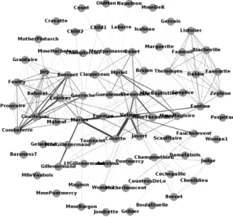
Since the world of concepts and techniques around social networks is very vast, before dealing with formal definitions and models, it is useful to start with an example that helps to give some ideas of what social networks are and how they can be modeled. The example we illustrate is a representation of the rela-tionships among the characters ofLes Misérables, a French historical novel by Victor Hugo published in 1862. Les Misérables, which is considered one of the greatest novels of the 19th century, follows the lives and interactions of several characters, in particular the struggles of ex-convict Jean Valjean, being the protagonist of the novel. The network of the relationships is shown in Figure
1.1. The data used to build the network are from [135]. The kind of represen-tation depicted in the figure is called social graph, where the circles, usually named nodes or vertices, are individuals, while the edges (or links) denote relationships between them. Moreover, in this particular case, the thickness of the edge depicts the intensity of the relationship between two nodes. The more the line is thick, the more the two nodes have a strong relationship. As simple reference instance, let’s look at nodes “Valjean” and “Cosette” at the center of the graph. Since Cosette is one of the character having a key role in the novel, and Valjean is her surrogate father, their relationship is quite intense, consequently their edge is rather thick. Similarly, we have other two strong relationships between node “Marius”, who is the suitor of Cosette, and Valjean and Cosette, respectively.
The just described example gives an idea of how a social network can be structured and what kind of characteristics it may have. Although a specific social network is usually pretty different from others, a common language able to describe, represent and measure all of them exists. We first start giving some fundamental definitions and properties of networks.
Definition 1. A Graph is defined as an object G pV, Eq, where V
t1, . . . , nu is the finite set of vertices or nodes, while E V V is the finite set of edges linking nodes. The two edges e pi, jq, e pj, iq PE (or, in an equivalent notation,ei,j, ej,i PE) if and only if a connection between nodesi
and j exists.
The canonical form of a network is the undirected graph, like the one de-picted in Figure1.1, in which two nodes are either connected or they are not.
Figure 1.1: “Les Misérables” social network
However, a directed version of the social graph also exists, usually called di-graph (i.e., directed graph). A digraph differs from an undirected graph for the presence of the directionality of its edges. In other terms, there are net-works in which one node may be connected to a second without the second being connected to the first. Therefore, an edge a pi, jq is considered to be directed if a link from i toj exists, where j is called the head and iis called the tail of the edge. For convenience, we refer to a digraph as D pV, Aq whereA is the finite set of directed edges or arcs. In what follows the default is that the network is undirected, and we explicitly use the word digraph, or the notation D pV, Aq, when a directed network is considered.
Concepts and properties of networks. Networks are usually evaluated and categorized on the basis of some properties. While in Section 1.1.1.3 we examine in detail the essential measures used in graph theory and social net-work analysis, here we introduce some preliminary concepts and properties of networks.
Size of the network and cardinality of the edge set. As already discussed, a graph is an object formed by a set of nodes and a set of edges. The cardi-nality of the node set, namely |V|, denotes the size of the network, while the cardinality of the edge set, i.e., |E| for graph or |A| for digraph, strictly de-pends on the number of nodes and the density of the network. The maximum
number of edges in an undirected graph without self-loops is |E| npn21q, while in the case of a digraph is |A| npn1q, where n |V| is the total number of nodes. The difference between |E|and |A|is obvious because in a digraph each pair of nodes pi, jq could have two arcs, while in an undirected graph there could be only one edge.
Weight. The weight of an edge wpeq denotes the intensity (or, in some cases, the cost or the length) of the relationship between the two nodesiandjin the edgee. A graph is a weighted graph if a weight is assigned to each of its edges [129]. Some authors call such a weighted graph anetwork [186]. However, we will use the world “network” as general term to refer to a graph or digraph. An example of weighted graph is the network shown in Figure 1.1.
Walks, paths and cycles. A walk in a networkG pV, Eq between two nodes i and j is a finite sequence of edges pi1, i2q,pi2, i3q, . . . ,piK1, iKq such that pik, ik 1q PE for each kP t1, . . . , K1u, with i1 iand iK j. Similarly,
the path is defined as the walk, but with the additional constraint that each node in the sequence i1, . . . , iK must be distinct. The shortest path between
nodesi and j is calledgeodesic, while the longest one is called diameter. Fi-nally, a cycle is a walk that starts and ends at the same node and such that all other nodes are distinct. Therefore, the only node that appears more than once is the starting/ending node.
Common network structures. There are some particular network structures that have specific names and properties. A tree is an acyclic connected net-work, namely a graph without any cycles. A forest is a network such that every component (see next paragraph) is a tree. A forest with n nodes and k components has nk edges [165]. A specific case of forest is the star. A star is a network in which every edge in the network involves a specific node i. Finally, acircle is a graph having a single cycle, in which every node in the graph has exactly two neighbors.
Connectivity, clique and components. In many applications (e.g., spread of disease) there is the need to track if a node can reach any other node. Such a feature is related to the property of connectivity. A network isconnectedif ev-ery pair of nodes is connected by some path in the network. From this concept we can define acomponent of a networkG pV, Eq as a nonempty connected subnetwork G1 pV1, E1q such that 0 V1 V and E1 E. Therefore, a connected component is a maximal connected subgraph of G. In the case of a digraph, there is the need to distinguish between weakly connected compo-nent and strongly connected compocompo-nent. A weakly connected component is a maximal subgraph of a directed graph such that, for every pair of nodes i
Figure 1.2: Two examples of networks: (a) undirected graph, (b) digraph
and j in the subgraph, there is an undirected path fromitoj and a directed path from j to i. Vice versa, a strongly connected component is a maximal subgraph such that, for every pair of nodes iand j in the subgraph, both the paths from itoj and from j toi are directed. Finally, it is definedcomplete network a network having all possible edges, so thatE Kk11zKk1 1pik, izq
in undirected graphs, and AKk11Kz1,z1kpik, izq in the case of digraphs.
A clique [148] in G pV, Eq is a subset of the vertex set C V such that for every pair of nodes in C, an edge connecting the couple exists. This is equivalent to saying that the subgraph induced byC is complete.
Neighborhood. Another fundamental concept of networks is the neighborhood. The neighborhood of a node i is the set of vertices that i is linked to. For-mally, we define the neighborhood of nodeibelonging to an undirected graph, as Npiq tj :ei,j 1u. If we are dealing with weighted networks, then we
define the neighborhood of i asNpiq tj :ei,j ¡0u. However, this notation
is not very common because it is a modification of the original definition just for weighted networks. In the case of digraph we cannot refer to the concept of neighborhood as in undirected graphs because of the directionality of edges. Thus, we define the set of successors as Spiq tj : ei,j 1u and the set of
predecessors asPpiq tj:ej,i1u.
1.1.1 Representation and measurement of networks
In this section we present some of the fundamentals on how networks are represented, measured and characterized. As we have already seen, in nature there are several kinds of networks, for this reason a general way does not exist to represent all of them. However, there are some representations widely used by many applications. Here we describe the two most popular ways of denoting networks.
The simplest formalism for representing a network is the adjacency list. An adjacency list is a collection of unordered lists, one for each vertex in the graph, describing the sets of neighbors. In other terms, the adjacency list of
nodeiis a list includingiin the first position and then all the nodes belonging to the i’s neighborhood: ti, j :jPNpiqu. Regarding digraphs, the adjacency list is defined considering the set of the successors: ti, j : j P Spiqu. The corresponding adjacency lists of the example graph shown in Figure 1.2a is the following:
t1,2,3u,t2,1,3,4u,t3,1,2u,t4,2u while the adjacency list of the digraph in Figure1.2b is:
t1,2,3u,t2,1,4u,t3,1,2u,t4u
Clearly, the two lists are different due to the different type of the two networks. For example, in the case of the digraph, node 4 does not have any successor, therefore its list is formed by only itself. Vice versa, in the undirected graph, node 4 has as neighbor node 2 in its adjacency list.
The main benefits of adjacency lists are compactness and used space, which is Opn mq, where n |V| and m |E|. However, because of its simple formulation, the main limitation of an adjacency list is the inability to add further details about the network it represents. For instance, no information about weights can be included.
Another common way to represent graphs is the adjacency matrix. An adjacency matrix Mis a nnsquare matrix, where the elementmi,j denotes
the relationship between nodes iand j. Thus, mi,j 1 if nodes i and j are
linked, mi,j 0 otherwise. Furthermore, in undirected graphs the equality
mi,j mj,i is always true. Therefore, the adjacency matrix of an undirected
graph is always symmetric, namely M MT. Vice versa, in digraphs it is likely that mi,j mj,i, so no assumption about symmetry can be done. The
adjacency matrix of the graph in Figure 1.2a is:
M 0 1 1 0 1 0 1 1 1 1 0 0 0 1 0 0
In the case a network is weighted, then the corresponding weighted adja-cency matrixWshould be considered, where each elementwi,j PR indicates
the weight of the edge pi, jq. The graph shown in Figure 1.2a is a weighted networks, so its weighted adjacency matrix is:
W 0 0.2 0.2 0 0.2 0 0.5 0.1 0.2 0.5 0 0 0 0.1 0 0
while the adjacency matrix of the weighted digraph shown in Figure1.2b is: W 0 0.1 0.35 0 0.2 0 0 0.1 0.05 0.2 0 0 0 0 0 0
Notice that, in both the cases, the diagonal of W has all the elements wi,i 0. This is due to the fact that, in our examples, we are considering
networks without self-loops. As opposed to adjacency lists, the adjacency matrix can represent weighted network; however, the space in memory to store a full adjacency matrix isOpn2q. This could be a serious problem when considering networks having million of nodes.
1.1.1.1 Network file-formats
The simplest file-format to represent a network is thecomma-separated values (CSV), which stores tabular data in plain-text form. A CSV file consists of a certain number of records, separated by line breaks, where each record consists of fields separated by some character, most commonly a literal comma or tab (in this case the format is sometimes called TSV, acronym of tabular-separated values). CSV is widely used in many applications, but at present a general standard formalizing it does not exist, even though RFC 4180 [24] provides a sort of guidelines. Among its requirements we find that a) each line (optional for the last line) must end with (CR/LF) characters, b) an optional header record may be included, c) each record must contain the same number of comma-separated fields, d) a field may be double-quoted, e) fields containing a line-break, double-quote, and/or commas should be quoted and f) a double quote character in a field must be represented by two double quote characters. The adjacency list relative to the undirected graph in Figure 1.2a can be stored in a CSV file in the following way:
1 1 ,2 ,3
2 2 ,1 ,3 ,4
3 3 ,1 ,2
4 4 ,2
while the adjacency matrix:
1 ,1 ,2 ,3 ,4
2 1 ,0 ,0.2 ,0.2 ,0
3 2 ,0.2 ,0 ,0.5 ,0.1
4 3 ,0.2 ,0.5 ,0 ,0
5 4 ,0 ,0.1 ,0 ,0
where the first row and the first column of the CSV-matrix denotes the header of the file containing the nodes IDs.
Another popular notation is GDF [7], the file format used by GUESS [15]. It is built like a CSV, but it supports attributes to both nodes and edges. A standard file is divided in two sections, one for nodes and one for edges. Each section starts with a header line, which basically is the column title. Below, the GDF file representing the graph of Figure1.2a:
1 nodedef > n a m e INT
2 1
3 2
4 3
5 4
6 edgedef > n o d e 1 INT , n o d e 2 INT , w e i g h t D O U B L E
7 1 ,2 ,0.2
8 1 ,3 ,0.2
9 2 ,3 ,0.5
10 2 ,4 ,0.1
Since GDF only lists nodes and existing edges with corresponding weights, the used space is Opn 2m tq, where t is related to the weight attribute. Clearly, if the file explicits other attributes, such as labels, the space increases, but it always remains linear.
Graph Modelling Language (GML) [12] was one of the first attempt to propose a common language to model graphs. Indeed, the main goal of the authors was developing a format platform independent, easy to implement and able to represent arbitrary data structures, where it would have been possible to attach additional information to every object. A GML file consists of hierarchically organized key-value pairs. A key is a sequence of alphanumeric characters, while a value is either an integer, a floating point number, a string or a list of key-value pairs enclosed in square brackets. Graphs are represented by the keys “graph”, “node” and “edge”. The topological structure is modeled with the node’s “id” and the edge’s “source” and “target” attributes. The GML representation of the graph in Figure 1.2a is the following:
1 g r a p h 2 [ 3 n o d e 4 [ 5 id 1 6 l a b e l "1" 7 ] 8 n o d e 9 [ 10 id 2 11 l a b e l "2" 12 ] 13 n o d e 14 [ 15 id 3 16 l a b e l "3" 17 ] 18 n o d e 19 [ 20 id 4 21 l a b e l "4" 22 ] 23 e d g e 24 [ 25 s o u r c e 1 26 t a r g e t 2 27 w e i g h t 0.2 28 ] 29 e d g e 30 [ 31 s o u r c e 1 32 t a r g e t 3 33 w e i g h t 0.2 34 ] 35 e d g e 36 [ 37 s o u r c e 2 38 t a r g e t 3 39 w e i g h t 0.5 40 ] 41 e d g e
42 [ 43 s o u r c e 2 44 t a r g e t 4 45 w e i g h t 0.1 46 ] 47 ]
GraphML [13] is another file-format for graphs. The main feature of GraphML is that it does not use a custom syntax, but it relies on XML [34]. The principal purpose of the authors was to make GraphML suit-able for all types of programs and services processing graphs. Its main fea-tures include support for directed, undirected, and mixed graphs, hyper-graphs, hierarchical hyper-graphs, graphical representations, references to external data, application-specific attribute data and light-weight parsers. The full GraphML syntax is defined by the GraphML schema [14]. Here, we just recap its basic elements. The file content is wrapped into a graphml ele-ment, while the whole network is included in the graph markup, in which it is also possible to set the graph type: <graph edgedefault="directed"> or<graph edgedefault="undirected">. Nodes are denoted by the element <node /> which usually includes the attribute id, and edges by the element <edge /> containing the attributes source and target. Finally, each at-tribute is defined in a key element with an identifier, a name, a title, the scope for edge or node, and the type of data. The GraphML representations of the graph in Figure 1.2a is the following:
1 <? xml v e r s i o n = " 1 . 0 " e n c o d i n g =" UTF -8" ? > 2 < g r a p h m l x m l n s=" h t t p :// g r a p h m l . g r a p h d r a w i n g . org / x m l n s " 3 x m l n s:xsi=" h t t p :// www . w3 . org / 2 0 0 1 / X M L S c h e m a - i n s t a n c e " 4 xsi:s c h e m a L o c a t i o n=" h t t p :// g r a p h m l . g r a p h d r a w i n g . org / x m l n s 5 h t t p :// g r a p h m l . g r a p h d r a w i n g . org / x m l n s / 1 . 0 / g r a p h m l . xsd "> 6 < key id=" d1 " for=" e d g e " a t t r.n a m e=" w e i g h t " a t t r.t y p e=" d o u b l e "/ > 7 < g r a p h id=" G " e d g e d e f a u l t=" u n d i r e c t e d "> 8 < n o d e id=" 1 " / > 9 < n o d e id=" 2 " / > 10 < n o d e id=" 3 " / > 11 < n o d e id=" 4 " / > 12 < e d g e s o u r c e=" 1 " t a r g e t=" 2 "> 13 < d a t a key=" d1 "> 0.2 </ data > 14 </ e d g e > 15 < e d g e s o u r c e=" 1 " t a r g e t=" 3 "> 16 < d a t a key=" d1 "> 0.2 </ data > 17 </ e d g e > 18 < e d g e s o u r c e=" 2 " t a r g e t=" 3 "> 19 < d a t a key=" d1 "> 0.5 </ data > 20 </ e d g e > 21 < e d g e s o u r c e=" 2 " t a r g e t=" 4 "> 22 < d a t a key=" d1 "> 0.1 </ data > 23 </ e d g e > 24 </ g r a p h > 25 </ g r a p h m l >
The last file-format we discuss is Graph Exchange XML Format (GEXF) [9]. GEXF is another XML-based language for describing graph structures, their associated data and dynamics. Indeed, with respect to previous for-mats, GEXF supports temporal dynamic networks. However, this feature will be better argued in Section 1.2.1.1 after introducing evolving networks. The GEXF project started in 2007 as reference network format for Gephi [8]. Its schema is defined in [10] where the 1.2 draft version is the recom-mended version to work with. As in GraphML, the graph structure is included in the element graph, and nodes and edges are denoted by <node /> and <edge />, respectively. The fundamental difference with respect to GraphML is the grouping of the two entities. Indeed, all nodes are included in the el-ement <nodes>...</nodes>, while all edges are grouped within the element <edges>...</edges>. Another important feature of GEXF is the default support for assigning weights to edges. Graphs in GEXF may be mixed as well. In other words, they can contain directed and undirected edges at the same time. The following code shows the GEXF representation of the graph in Figure 1.2a: 1 <? xml v e r s i o n = " 1 . 0 " e n c o d i n g =" UTF -8" ? > 2 < g e x f x m l n s=" h t t p :// www . g e x f . net / 1 . 2 d r a f t " x m l n s:xsi=" h t t p :// www . w3 . org / 2 0 0 1 / X M L S c h e m a - i n s t a n c e " xsi: s c h e m a L o c a t i o n=" h t t p :// www . g e x f . net / 1 . 2 d r a f t h t t p :// www . g e x f . net / 1 . 2 d r a f t / g e x f . xsd " v e r s i o n=" 1.2 "> 3 < g r a p h m o d e=" s t a t i c " d e f a u l t e d g e t y p e=" u n d i r e c t e d "> 4 < nodes > 5 < n o d e id=" 1 " / > 6 < n o d e id=" 2 " / > 7 < n o d e id=" 3 " / > 8 < n o d e id=" 4 " / > 9 </ n o d e s > 10 < edges > 11 < e d g e s o u r c e=" 1 " t a r g e t=" 2 " w e i g h t=" 0.2 " / > 12 < e d g e s o u r c e=" 1 " t a r g e t=" 3 " w e i g h t=" 0.2 " / > 13 < e d g e s o u r c e=" 2 " t a r g e t=" 3 " w e i g h t=" 0.5 " / > 14 < e d g e s o u r c e=" 2 " t a r g e t=" 4 " w e i g h t=" 0.1 " / > 15 </ e d g e s > 16 </ g r a p h > 17 </ g e x f >
1.1.1.2 Software tools to analyze complex networks
Nowadays, the analysis of complex networks requires to analyze several metrics introduced in graph theory and in Social Network Analysis (SNA). However, before starting to measure a specific metric, sometimes it is useful to visually analyze the raw data. Indeed, thanks to the visualization, humans can easily find patterns in network structures as well as have a first visual perception of
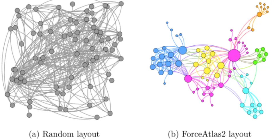
the network structure. In Figure 1.3 we can see, for instance, two different ways of visualizing the same network of Les Misérables. Specifically, Figure
1.3a shows the network using a random layout, while Figure 1.3b arranged the graph through the ForceAtlas2 layout [124]. It appears quite obvious that the amount of information provided by Figure 1.3b is higher than the one provided by the randomly drawn graph. However, this kind of analysis usually requires an exploratory process [171]. Already in 1996, Scheiderman [181] summarizes the general process steps of graph visualization: “Overview first, zoom and filter, then details-on-demand”. Therefore, in order to satisfy the requirements for such a process, visualization tools should support high quality layout algorithms, data filtering, clustering, statistics and visualization features.
(a) Random layout (b) ForceAtlas2 layout
Figure 1.3: Two different kinds of visualizations of the network Les Misérables: (a) shows a representation using a random layout, while (b) employs the ForceAtlas2 layout [124] where nodes are resized according to their degree and colored according to their maximum modularity class.
In the following we briefly list and introduce the most popular software tools and libraries for visualizing and analyzing complex networks.
• NetworkX [20] is a Python software package for creating, manipulating and studying structures and dynamics of social, biological, and infras-tructure networks. NetworkX includes several mechanisms to easily work with graphs and, at present, is one of the most popular libraries among researchers.
• iGraph [16] is another software package that can be programmed in R, Python and C/C++. It includes a collection of network analysis tools with the emphasis on efficiency, portability and ease of use.
• R[28] is a language and environment for statistical computing and graph-ics. Due to its statistical nature, it is very used in the research commu-nity to study and analyze networks.
• D3.js [4] is a JavaScript library for manipulating documents based on data. It is one of the most recent tools available to work with raw data in order to transform them into a structured format.
• sigmajs [25] is another JavaScript library dedicated to graph drawing. It makes easy to publish networks on the Web and allows developers to integrate network exploration in rich Web applications in order to make network manipulation smooth and fast for the user.
• GUESS [15, 43] is a visualization and analysis tool based on Gython, a domain-specific embedded language which supports operators for di-rectly working on graph structures in an intuitive way.
• Pajek [23,57] is one of the first visual exploratory tools for graph visu-alization and analysis. It is freely available for noncommercial use.
• Cytoscape [3,180], shown in Figure1.4, is an open source software plat-form for visualizing and analyzing molecular interactions and biological networks. Cytoscape was originally designed for biological research, now it is a general platform for complex network analysis and visualization. At present, it is one of the most powerful tool for network analysis.
• Gephi [8,56] is one of the youngest graph-viz projects for the manipu-lation and visualization of complex networks. Specifically, it is an open source software based on the NetBeans platform (netbeans.org), spe-cialized in graph analysis and visualization thanks to several statistical plug-ins and a 3D render engine that speeds up the exploration and real-time rendering. In addition, one of the most powerful features of Gephi is the timeline component that allows to dynamically explore evolving networks. Gephi runs on Windows, Linux and Mac OS X and it is open-source and free. A screenshot of the main user interface is shown in Figure 1.5. Actually, Gephi has been our favorite tool to draw and measure networks throughout our research activity.
• Gexf4j [11] is a Java library to create and write GEXF files which can be used to visualize graphs in Gephi or other GEXF-supporting application. Gexf4j was initially designed by Javier Campanini and released under the Apache License 2.0. However, the Campanini’s release only supported the old GEXF schema (1.1 draft), so in 2012 we decided to take over the project, under the same license, and develop future versions. At present,
Figure 1.4: Cytoscape Figure 1.5: Gephi
gexf4j is continuously maintained and updated and the source code is hosted on Github [11]. The binary releases are published on Maven Central Repository [18] so that any Java developer can easily include gexf4j in her own Maven projects. In 2014 the library was downloaded more than 1000 times from Maven, while the Github repository has been cloned thousand and thousand of times since the beginning of the project.
1.1.1.3 Network measures
In mathematics and computer science, graph theory is a research area study-ing properties of graphs. We have seen that networks can be visualized and analyzed thanks to software tools, but, to make this possible, topological mea-sures describing the main structural properties of the graph [198,86,123] have to be investigated. In the following we review some of them.
Degree. One of the basic metrics of graph theory is the degree. Let G
pV, Eq be a non-empty graph, where V t1, . . . , nu is the node set and E V V the edge set. We have seen that the neighborhood of a vertexiinGis denoted as Npiq. Then, thedegree of node i, denoted dpiq, is:
dpiq |tj:ei,j1u| |Npiq|
In other words, the degree of node i is the number of its incident edges. A vertex of degree 0 is called isolated. If all the vertices of G have the same degree k, then G is called k-regular and we can speak of the degree of the graph. In the case of a digraph D pV, Aq, the degree of a node i is the sum of the in-degree, defined as dpiq |Ppiq| and the out-degree, namely d piq |Spiq|. A vertex i having dpiq 0 is called source, while a vertex withd piq 0 is calledsink.
Sometimes, in addition to analyze the single node degrees, it is also useful to examine the average degree of the graph to better understand what kind of structure shapes the network. Thus, the number
dpGq 1
|V|
¸ iPV
dpiq
denotes theaverage degreeofG. This quantity can be also expressed asεpGq
2|E|
|V|. Indeed, counting all the nodes degrees in Gis equivalent to count twice
every edge:
2|E| ¸
iPV
dpiq (1.1)
(1.1) is called degree sum formula and from which it follows that:
εpGq dpGq
This leads to the following proposition, sometimes namedhandshaking lemma.
Proposition 1. The number of vertices of odd degree in a graph is always even.
Proof. A graphG has 12°iPV dpiq edges, so °dpiq is an even number.
Clearly, in the case of digraphs, if we split the degree in in-degree and out-degree, then the degree sum formula becomes:
|A| ¸
iPV
dpiq ¸
iPV
d piq
However, if we consider the total degree dpGq as the sum of in-degree and out-degree: ¸ iPV dpiq ¸ iPV dpiq ¸ iPV d piq
then we get back to (1.1). Lastly, if for every nodeiPV we haved piq dpiq, then the graph is called balanced digraph.
Weighted degree. If we now focus on weighted networks, a fairer metric to consider is the weighted degree, sometimes callednode strength. The weighted degree is defined similarly to the degree, but the weighted version also takes into account the weight of incident edges. Let G pV, Eq be a non-empty weighted graph, where V t1, . . . , nu is the node set and E V V is the
edge set. Then, W is the nn adjacency matrix of G having a weight wi,j
on each edge pi, jq. Thus, the weighted degree of node iis defined as: wdpiq ¸
jPNpiq
wi,j
In other terms, the weighted degree of a node is the sum of weights of the edges incident on that node. As for digraphs, the weighted in-degree and out-degree are defined by just replacing Npiq with Ppiq and Spiq to the previous formula, respectively.
Density. Another fundamental metric giving an idea on the structure of the graph is the density. Let G pV, Eq be a non-empty graph, where V
t1, . . . , nu is the node set andE V V is the edge set. The cardinality of V is |V| n, while the total number of edges inE is |E| m. We recall that the maximal number of edges of E is npn21q. Therefore, we define the density as the fraction of existing edges inE, namely m, and the maximal number of edges of the graph:
λpGq 2m npn1q
In the case of a digraph D pV, Aq, being npn1q the maximal number of arcs in A, the density is:
λpDq m npn1q
Clustering coefficient. The clustering measures the tendency of the neigh-bors of a node ito be connected to each other. In other terms, theclustering coefficient [199] is a measure of the degree to which nodes in a graph tend to cluster together. LetG pV, Eqbe a non-empty graph, whereV t1, . . . , nu is the node set and E V V is the edge set. The clustering coefficient ϑpiq of a nodei is computed as the ratio between the actual number of edges between its neighbors and the value of the maximum possible edges in the neighborhood Npiq:
ϑpiq 2|tev,u :v, uPNpiqu|
|Npiq|p|Npiq| 1q
This measure is meaningful only for|Npiq| ¡1. If|Npiq| 1 then we consider ϑpiq 0. If we now look at a digraph D pV, Aq, since the number of the maximum possible arcs in the neighborhood Npiq is |Npiq|p|Npiq| 1q, the clustering coefficient of nodeiis:
ϑpiq |tav,u :v, uPNpiqu|
|Npiq|p|Npiq| 1q
The clustering coefficient of the network, which measures the overall degree of clustering of the graph, is defined as the average on the local clustering coefficients of all the vertices:
xϑy 1 n n ¸ i1 ϑpiq wheren |V|is the total number of nodes.
Modularity. The main difference between a completely random graph and a real-world social network is that the latter often exhibits interesting properties regarding its corresponding structure. One of these features is the community structure, namely the division of nodes into groups within which the network connections are dense, but between which they are sparser. This property is better known asmodularity[161,160]. Its name derives from the measurement of the division of the network into “modules” (or communities).
Consider a network divided inkcommunities. LetWbe akksymmetric matrix whose elementwi,j is the fraction of all edges in the network that link
nodes in communityito nodes in communityj. We can define the modularity as: Q¸ i wi,i ¸ j wi,j 2
where Q lies in the range r0.5,1q. This quantity measures the fraction of the edges in the network that connect nodes in the same community minus the expected value of the same quantity in a network with the same commu-nity divisions but random connections between the nodes. A value of Q ¤0 indicates a random behavior of the network, while values approachingQ1, which is the maximum, indicate strong community structure.
Centrality. One of the most important indicator in SNA is thecentrality, that is a measure able to identify the most influent vertices within a social network. In other terms, centrality indices have a duty to answer the follow-ing question: “What characterizes an important vertex?”. Actually, the word “important” has different meanings, depending on the considered context. For this reason, several centrality indices exist [103, 67, 68], such as degree cen-trality, closeness cencen-trality, betweenness centrality and eigenvector centrality. Other two famous indices of centrality are Katz centrality [130] and Pagerank
[164].
The degree centrality is the historically first and conceptually simplest in-dex belonging to the centrality class. It indicates how well a node is connected in terms of direct1 connections. Let G pV, Eqbe a non-empty graph, where V t1, . . . , nuis the node set with cardinality|V| nand E V V is the edge set. The degree centrality of a node iis simply:
Cdpiq
dpiq n1
Of course, the degree centrality misses a lot of other aspects of a network. For instance, it does not measure how well-located a node is in a network. In other words, a node with a high degree centrality could be located at the border of a graph and linked to a certain number of nodes already well-linked to other vertices, and thus having low relevance in terms of structure, while another node with low degree centrality could be located in the middle of the network linking two subgraphs, and so being more important for the connectivity of the whole graph.
As usual, in the case of digraphs, we must diversify between in-degree and out-degree centrality. However, the concept remains the same.
The closeness centrality measures how close a given node is to any other node. In other words, the closeness centrality of a node i is the reciprocal of the sum of the geodesics from i to all n1 other nodes. Since the sum of distances depends on the number of nodes in the graph, closeness is normalized by the sum of the minimum possible distancesn1:
Ccpiq
n1
°n1
j1,ij`pi, jq
where`pi, jq is the number of links in the geodesic betweeniand j.
An index of centrality that better measures how well situated a node is in terms of the paths in which it acts as a bridge is thebetweenness centrality. It quantifies the number of times a node lies two other nodes along geodesics. It was proposed by Freeman [102] as a measure for quantifying the control of an individual on the communication between other humans in a social network. Let σpiqk,j denote the number of geodesics between k and j that i lies on,
and let σk,j be the total number of shortest paths between k and j. We can
estimate how central a node i is in terms of connecting two other nodes by
1
In this context, the word “direct”, which is different from “directed”, does not refer to the directionality of edges, but to all those links directly incident on a node.
computing the ratio σpiqk,j
σk,j . Averaging this ratio across all pairs of nodes, the
betweenness centrality of a node iis:
CBpiq ¸ kj,iRk,j σpiqk,j{σk,j pn1qpn2q 2
wheren |V|is the total number of nodes.
The eigenvector centrality is another measure of node’s influence proposed by Bonacich [65]. The basic idea is that the centrality of a node is proportional to the sum of the centrality of the vertices in its neighborhood Npiq. For a given graph G pV, Eq, let M be the adjacency matrix, so that mi,j 1
if node i is linked to node j, namely i and j are neighbors, and mi,j 0
otherwise. The eigenvector centralityCEpiqof node iis defined as:
CEpiq 1 λ ¸ jPNpiq mi,jCEpjq
or equivalently, in matrix notation:
λCEM CE (1.2)
where eigenvalueλworks as a proportionality factor. (1.2) identifies the eigen-vector equation (see AppendixA.1for background on eigenvectors and eigen-values), in whichCEis a right (or column) eigenvector. Generally, there could be many different eigenvaluesλfor which an eigenvector solution exists. How-ever, the requirement of all the entries in the eigenvector must be positive implies (by the Perron–Frobenius theorem [173, 107], Perron root) the exis-tence of a real positive eigenvalue λ strictly greater in absolute value than all other eigenvalues, so it must be the largest eigenvalue of M, and CE the corresponding eigenvector. One method to compute the eigenvector centrality is Power iteration [155] (see Appendix A.2for further information).
A variant of the eigenvector centrality is theKatz centrality, which quanti-fies the number of all nodes that can be connected through a path, penalizing the contribution given by distant nodes. It is a generalization of the degree centrality which instead measures the number of direct neighbors. For a given graphG pV, Eqwith|V| nthe number of nodes in the network, let Mbe the adjacency matrix. The Katz centrality is defined as:
CKpiq 8 ¸ k1 n ¸ j1 αkpMkqj,i
whereα is an attenuation factor ranging between 0 and 1. The k-th power of
Mgives an adjacency matrix of a graph with the same vertex set and an edge between two vertices if and only if there is a path of length at mostkbetween them [100].
PageRank. In recent years, one of the most important measure of nodes’ centrality in static networks has certainly beenPageRank[164,140]. The basic metaphor behind PageRank [69] considers arandom surfer that starts from a randomly chosen web page. At every page she visits, the random surfer either gets bored and quits navigation with a fixed probability, or she selects one of her outgoing neighbors uniformly at random. If the page has no outgoing links (i.e., it is asink),the surfer jumps to a page selected uniformly at random in the network. The rank of a page according to the PageRank algorithm is the probability that a random surfer stops at that page. We denote by α the probability that the surfer continues her random walk (the damping factor). We must highlight that PageRank is usually used in digraphs, where the directionality of edges is fundamental for the algorithm. Vice versa, in undirected graphs, it can be shown that PageRank is statistically close to the degree distribution of the graph [172].
Let Npiq be the set of neighbors of a node iand dpiq |Npiq| the degree of i. The transition matrix [179, p. 114] Qof Gis defined as follows:
qi,j #
1
dpiq, ifdpiq 0 and jPNpiq;
0, otherwise.
In addition, we denote by A the modified transition matrix of G, corre-sponding to removal of sinks, namely the stochastic matrix such thatai,j qi,j
ifiis not a sink, ai,j 1n otherwise.
Given these definitions, the Pagerank vector π of Gis the stationary dis-tribution (equivalently, the main left eigenvector) of the ergodic Markov chain [179, Theorem 4.2, p. 119] corresponding to the following stochastic matrix:
P:αA p1αq n111T, where1 denotes the 1-value column vector, while
1T is the row vector with unit components.
A more extensive discussion about PageRank is given in Chapter 3, in which we will also describe further issues.
1.2
Social networks in dynamic contexts
So far, we focused our attention on static networks, i.e., graphs that do not change over time. An advanced class of graphs is that of evolving networks. This kind of networks are networks that change as a function of time. For this reason, they are sometimes called time-evolving networks [146] or temporal