Daniele Buono
IBM T.J. Watson [email protected]Fausto Artico
IBM T.J. Watson [email protected]Fabio Checconi
IBM T.J. Watson [email protected]Jee W. Choi
IBM T.J. Watson [email protected]Xinyu Que
IBM T.J. Watson [email protected]Lars Schneidenbach
IBM T.J. Watson [email protected]ABSTRACT
A recent advancement in the world of heterogeneous computing, the NVLink interconnect enables high-speed communication be-tween GPUs and CPUs and among GPUs. In this paper we show how NVLink changes the role GPUs can play in graph, and more in general, data analytics. With the technology preceding NVLink, the processing efficiency of GPUs is limited to data sets that fit into their local memory.
The increased bandwidth provided by NVLink imposes a re-assessment of many algorithms—including those used in data analytics— that in the past could not efficiently exploit GPUs because of their limited bandwidth towards host memory.
Our contributions consist in the introduction of the basic proper-ties of one of the first systems using NVLink, and the description of how one of the most pervasive data analytics kernels, SpMV, can be tailored to the system in question. We evaluate the resulting SpMV implementation on a variety of data sets, and compare favorably to the best results available in the literature.
ACM Reference format:
Daniele Buono, Fausto Artico, Fabio Checconi, Jee W. Choi, Xinyu Que, and Lars Schneidenbach. 2017. Data Analytics with NVLink: An SpMV Case Study. InProceedings of CF’17, Siena, Italy, May 15-17, 2017,8 pages. DOI: http://dx.doi.org/10.1145/3075564.3075569
1
INTRODUCTION
We examine the impact of NVLink—a fast and improved alterna-tive to the traditional Peripheral Component Interconnect Express (PCIe) to connect GPUs and CPUs—on the viability and performance of large-scale data analysis on GPUs. We use sparse matrix-vector multiply (SpMV) as a proxy application, since it is arguably the biggest performance bottleneck for many classes of data analysis al-gorithms, to show that NVLink eliminates many of the barriers that have prevented GPUs from being more widely used for large-scale analytics.
To first order, streaming the matrix dominates SpMV perfor-mance since SpMV is largely memory bandwidth-bound. This, cou-pled with the fact that GPUs are memory bandwidth-rich, makes
Permission to make digital or hard copies of all or part of this work for personal or classroom use is granted without fee provided that copies are not made or distributed for profit or commercial advantage and that copies bear this notice and the full citation on the first page. Copyrights for components of this work owned by others than ACM must be honored. Abstracting with credit is permitted. To copy otherwise, or republish, to post on servers or to redistribute to lists, requires prior specific permission and/or a fee. Request permissions from [email protected].
CF’17, Siena, Italy
© 2017 ACM. 978-1-4503-4487-6/17/05. . . $15.00 DOI: http://dx.doi.org/10.1145/3075564.3075569
GPUs highly attractive for speeding up data analysis. With the explosion of data from social networks, online shopping, ubiqui-tous sensors, and more, analyzing large amounts of data in a timely manner may evennecessitatethe use of GPUs in the near future. However, the low PCIe memory-bandwidth between the CPU and the GPU makes it extremely difficult to amortize the cost of mov-ing data from CPU memory to GPU memory before computation. Moreover, the use of faster, but more expensive HBM2 (High Band-width Memory) technology severely limits the total memory size on GPUs, further making it difficult to use GPUs for extremely large data sets.
Prior works have explored the use of GPUs for large-scale data analysis indistributedsettings—where network latency and band-width palliate the PCIe problem—to achieve non-trivial speedup over CPU-only solutions. Nevertheless, the low PCIe bandwidth continues to prevent GPUs from reaching their full potential for large-scale data analysis. NVLink changes this paradigm by provid-ing much higher bandwidth between GPUs and their host CPUs, and among GPUs than previously available. On the system we used in our experiments, the overall bandwidth between GPUs and main memory is comparable to that available from the CPUs, making it possible to change the programming paradigm for data analytics.
Contributions and Findings.As far as we are aware, this is the first paper that explores the performance impact of NVLink on SpMV, and, in general, shows the results of running a data analytics kernel on a graph larger than the GPU memory footprint without paying any penalties for the streaming of data into the GPUs. We also provide a description of one of the first systems using NVLink, and the results of some microbenchmarks running on it.
Paper Layout.In Section 2, we describe the overall system ar-chitecture, focusing particularly on the NVLink specification and NVIDIA’s new Pascal microrachitecture. In Section 3, we discuss the role of SpMV in large-scale data analytics, as well as our proposed implementation. We present our experimental result in Section 4 and consider previous and related work in Section 5. Finally, we conclude our paper in Section 6.
2
SYSTEM ARCHITECTURE
2.1
Hardware Platform
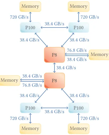
We use an IBM Power S822LC for HPC node, comprising 2 POWER 8 processor chips and 4 NVIDIA Tesla P100 (Pascal) GPUs. Our evaluation revolves around the use the system does, first of its kind, of NVLink Version 1.0 to connect the POWER 8 CPUs to the GPUs. An architectural overview of system connectivity is shown in Figure 1.
P8
P100 P100
P8
P100 P100
Memory Memory
Memory Memory
Memory
Memory
38.4 GB/s
38.4 GB/s 38.4 GB/s
38.4 GB/s 38.4 GB/s
38.4 GB/s
38.4 GB/s
720 GB/s 720 GB/s
720 GB/s 720 GB/s
76.8 GB/s
38.4 GB/s
76.8 GB/s 38.4 GB/s
Figure 1: Architecture of a Power S822LC for HPC Node. Each NVLink connection between CPU and GPU or GPU and GPU has an aggregate theoretical peak bandwidth of 38.2 GB/s in each direction.
NVLink uses the High-Speed Signaling Interconnect from NVIDIA to transmit data at a bandwidth of 19.2 GB/s in each direction. On our system, 2 links are installed between each GPU and its host CPU, and between the GPUs sharing the same socket. For each of those 2-link connections, the overall bandwidth is 38.4 GB/s, full-duplex.
The POWER 8 sockets are connected to each other by an SMP link capable of a theoretical peak 38.4 GB/s. Each POWER 8 socket can read from its local memory at 76.8 GB/s, and write to it at 38.4 GB/s.
Each POWER 8 CPU has 10 cores that run at 3.424 GHz. Each core has 64 KB of data cache, 32 KB of instruction cache, 512 KB of L2 cache and 8 MB of L3 cache. Each core supports up to 8 hardware threads. The power consumption of each chip is 190 W. Each socket has 512 GB of DRAM memory. In our experiments, the operating system is Red Hat Enterprise Linux Server version 7.3 Maipo.
The software environment and other architectural features of the PASCAL GPUs are reported in Table 1. The Streaming Multipro-cessors (SM) run at 1480 MHz, the High Bandwidth Memory (HBM)
runs at 715 MHz providing a GPU Global Memory theoretical band-width of 720 GB/s. Each GPU consumes 300 W. The NVIDIA Cuda compiler driver version is 8.0.55.
CUDA Driver Version / Runtime Version 8.0 / 8.0 CUDA Device Capability 6.0
Global memory (MB) 16,281 Streaming Multiprocessors (SM) 56 Single Precision CUDA Cores per SM 64 Double Precision CUDA Cores per SM 32 Load and Store Units per SM 16 Special Function Units per SM 16 Number of Instruction Caches per SM 1 Number of Instruction Buffers per SM 2 Number of Warp Schedulers per SM 2 Number of Dispatch Units per SM 4 Shared Memory Available per Block 48 KB
32-bit Registers Available per SM 64 KB Read-Only Data Cache per SM 64 KB Maximum SM Clock Frequency 1480 MHz Maximum Global memory Clock Frequency 715 MHz
Memory Bus Width 4096 bits Theoretical Global memory Bandwidth 720 GB/s
L2 Cache Size 4 MB
Total Quantity of Constant Memory 64 KB Warp Size in Number of Threads 32 Maximum Number of threads per SM 2048 Maximum Number of Threads per Block 1024
Table 1: Architectural Features of Pascal GPUs.
2.2
NVLink Performance
We proceed to characterize the performance of NVLink in what concerns our study on data analytics. We focus on CPU to GPU transfers, as they are the main bottleneck in our SpMV case study. To this end, we implemented a benchmark that stresses the NVLink capabilities with different transfer options and sizes, to measure the effective bandwidth we can achieve from an application.
The benchmark creates an MPI rank per GPU; because of the NUMA nature of the architecture, we bind each rank to the socket hosting the target GPU. Each rank allocates a certain number of blocks of a specified transfer size; the number of blocks is deter-mined experimentally to guarantee that we sample a sufficiently long execution time. The memory is initialized using random num-bers.
Memory on the host can be allocated in two different ways: a) pinned, and b) pageable. Pageable memory is the default alloca-tion policy of most operating systems, including Linux; it can be allocated with malloc in C or the operator new in C++. Pageable memory can be swapped and therefore moved during execution. Since the memory is allowed to move during a DMA copy, the sys-tem must first copy the CPU data into a CPU sys-temporary buffer, then transfer the buffer to a temporary GPU buffer and finally copy the data to the destination buffer on the GPU. This obviously increases both the latency and the bandwidth consumption.
will maintain the same physical addresses for the entire execution, allowing the system to optimize memory transfers: GPUs can copy data directly, and the memory is allocated as write-combined, to allow the CPU to efficiently read the area during transfers.
In addition to the different traffic pattern, CUDA does allow to execute asynchronous transfers only with pinned memory.
The benchmark is executed with different block sizes to identify the minimum transfer size required to achieve full bandwidth. The results of the experiments are shown in Figures 2a and 2b, for pageable and pinned memory respectively.
Because of the synchronous behavior and the additional traffic, the effective bandwidth per GPU is only 10−11 GB/s when using pageable memory. Pinned memory, on the other hand, can generate approximately 3×more bandwidth, with a per-GPU bandwidth of ∼30GB/sand an aggregate bandwidth of∼120GB/s, i.e. 80% of the peak CPU bandwidth.
Using the same benchmark we also verified that we can achieve full bandwidth with a limited number of asynchronous streams. This is important for our SpMV code since we plan to use only two streams during the execution (one computing, the other transfer-ring).
In terms of block sizes, the experiments shows that we can reach peak bandwidth with transfers larger than 4MB, both for pinned and pageable memory.
3
SPARSE MATRIX-VECTOR MULTIPLY
Sparse Matrix-Vector Multiply (SpMV) is one of the most fundamen-tal operations in linear algebra because sparse matrices are widely used to represent data in many domains, including computational simulation, machine learning, and graph analysis.
In its simplest format, as shown in Equation 1, SpMV defines a product operation between a sparse matrixA(m×n) and a dense column vectorxof sizen, and produces a dense vectorbof sizem.
bi = nX−1
k=0
Ai k ∗ xk (i=0,1, ...,m−1) (1)
The implementations of SpMV vary based on how the matrix is stored. As opposed to dense matrices, where the format is fixed and straightforward, researchers introduced different formats for sparse matrices that better fit either the sparsity pattern of the matrix or the characteristics of the system used to compute the multiplication. Among them, Compressed Sparse Row (CSR) is the de factostandard for general sparse matrices because of its limited footprint and the relatively high performance on general purpose architectures.
3.1
CSR-based SpMV
In CSR, the matrixAis stored using three contiguous arrays. The valarray contains the values of each non-zero element of the matrix ordered by rows. A second array, calledrowstart, points to the first element of each row inval. Since elements invalare ordered by row, all the elements invalbetweenrowstart[i] androwstart[i+1]
belong to rowiof the matrix. Finally, for each element inval, a corresponding element exists incolidxto denote the column of the element.
Using this representation, a straightforward implementation of SpMV is described in Algorithm 1.
Algorithm 1:CSR-based SpMV Algorithm.
Input:(rowstart,colidx,val): matrixA; x: input vector.
Output:b: output vector, initialized to 0.
1 fori←0tom−1do
2 forj←rowstart[i]torowstart[i+1]−1do
3 k←colidx[j];
4 b[i]←b[i]+(val[j]∗x[k]);
The algorithm scans sequentially the rows ofA. For each row, it pulls out all the non-zero elements of the matrix fromval[j] and multiplies them with the corresponding values of the vectorx[k]. Then, the accumulation is written intob[i]. One of the advantages of this implementation is that it sequentially reads the arrays com-posing the matrix, and it sequentially writes to the vectorbso that the accumulation can be performed by using a register.
3.2
Streaming SpMV over NVLink
GPUs are well suited for structured computation, such as dense lin-ear algebra, but require some programming effort to handle SpMV kernels efficiently. The irregularity of sparse matrices raises multi-ple challenges on memory coalescing, load balancing and thread divergence. For this reasons, most of the current efforts at efficient SpMV for GPUs target alternative format representations [2],[5], [7], [11], [12] and [15].
With our streaming SpMV implementation, however, we decided to not focus our efforts in creating yet another sparse format, for the following reasons:
• The cornerstone of most GPU-oriented formats is to find ways of making the structure of the matrix more regular, to reduce thread divergence and allow memory coalesc-ing; while this approach works for sparse but structured matrices (such as matrices from the PDE domain), this is generally ineffective on graphs, because of their natural absence of structure [2],
• GPU-oriented algorithms generally have an increased mem-ory footprint w.r.t. the CSR format; this effect is aggravated in graph matrices because of their absence of structure, as demonstrated in [4], where the authors showed that com-monly used formats like ELL or BCSR may require orders of magnitude more space than a simple CSR.
• In our streaming algorithm we plan to compute and trans-fer data concurrently; in this scenario, we expect the data transfer to be the bottleneck of the kernel, making GPU kernel efficiency a secondary point as it is unlikely to affect the final performance.
HostToDevice
1e+02 1e+05 1e+08
0 10 20 30 40
Block Size (Bytes)
Aggregate Bandwidth (GB/s)
factor(GPUS) 1 2 3 4
(a) Pageable Memory, Single CUDA Stream, Sync.
HostToDevice
1e+02 1e+05 1e+08
0 25 50 75 100
Block Size (Bytes)
Aggregate Bandwidth (GB/s)
factor(GPUS) 1 2 3 4
(b) Pinned Memory, Multiple CUDA Streams, Async.
Figure 2: Measured Host to Device NVLink Transfer Bandwidths
x
B0,0 B0,1 B0,2 B0,3
B1,0 B1,1 B1,2 B1,3
B2,0 B2,1 B2,2 B2,3
B3,0 B3,1 B3,2 B3,3
G0
G1
G2
G3
b0
b1
b2
b3
S0 S1
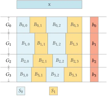
Figure 3: Block Layout for the SpMV Implementation. Each block-row is assigned to a different GPU, and within each block-row two streams are active per GPU. Since blocks and partitions are balanced using the nnz elements, the number of rows and columns per block may vary.
3.2.1 Blocking Scheme.Figure 3 shows the layout of the blocks across GPUs. The matrix is partitioned in 4 block-rows, each as-signed to a different GPUs. Each partition is then divided into blocks. Each block span for the entire set of rows and a subset of the columns assigned to the partition. To maintain the work among GPUs and blocks balanced, each partitions and each block will con-tain approximately the same number of elements. Depending on the structure of the matrix this may result in a different number of rows or columns per block. The input vector resides in host memory, and each GPU accesses it across the NVLink when needed. The partitioning scheme allows each GPU to make progress on a separate section of the output vector without the need for inter-GPU synchronization. A single synchronization is introduced, at the end of the SpMV computation, to transfer the output vector back to the host memory.
Algorithm 2 shows the algorithm to coordinate the execution of the SpMV kernels local to each GPU. Each GPU executes the presented pseudo-code in parallel on a different block-row of the input matrix to calculate a different section of the output vector. We assume each GPUGhas two local buffers for the input matrix and vector,xGi andA
G
i withi=0,1, to perform double-buffering,
and a single local copybGof the output vector (since we perform one computation at a time, from alternating streams). To guarantee maximum overlap, most of the operations are asynchronous, and each buffer pair is assigned to a separate streamSi. For simplicity,
the pseudo-code assumes an even number of blocks per row. In the pseudo-code,Bis an array of descriptors that stores in-formation about the blocks assigned to the GPU. Thecusparse -implementation of SpMV performs the update operation at lines 7 and 14.
3.2.2 Performance Model.
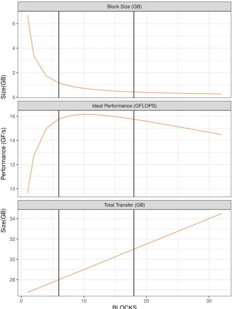
Selecting the proper block size (and number of blocks) for the streaming algorithm is not a trivial task. There is, of course, a phys-ical limitation imposed by the total amount of memory available on the GPU. But every block size below the memory limit is an admissible choice.
In fact, from a performance point of view, having more blocks improves the streaming effect since it allows the application to reach a steady state faster and keep it for a longer period of time. On the other hand, however, having too many blocks hurts performance because it increases the size of the CSR index.
To better understand the behavior of the streaming algorithm, we developed a simple analytical model that predicts the performance of SpMV depending on the number (and size) of blocks used.
Algorithm 2:Blocked SpMV.
Input:A: matrixA; x: input vector; B: blocking descriptors; S: CUDA stream descriptors
Output:b: output vector.
1 cudaMemcpy(bG,b,b.size);
2 cudaMemcpy(x0G,x,B0.x bytes); 3 cudaMemcpy(AG0,A,B0.nnz bytes); 4 i←0;
5 whilei<num blocksdo
6 {Multiply onS0and copy onS1.}
7 bG←AG0xG0 ;
8 cudaMemcpyAsync(xG1,x,Bi.x bytes,S1); 9 cudaMemcpyAsync(AG1,A,Bi.nnz bytes,S1);
10 i←i+1;
11 cudaStreamSynchronize(S0); 12 cudaStreamSynchronize(S1);
13 {Multiply onS1and copy onS0.}
14 bG←AG1xG1 ;
15 ifi<num blocksthen
16 cudaMemcpyAsync(x0G,x,Bi.x bytes,S0);
17 cudaMemcpyAsync(AG0,A,Bi.nnz bytes,S0);
18 i←i+1;
19 cudaStreamSynchronize(S0);
20 cudaStreamSynchronize(S1);
21 cudaMemcpy(b,bG,b.size);
We can see that every size fits on the GPU, so we may be tempted to use a single block and avoid streaming entirely, because this solution would be optimal in terms of total transfers from the CPU. However, with a single block, we cannot overlap computation and communication. Similarly, when we have a very limited number of blocks (i. e. 2 or 4), the cost of computing the last kernel impacts the execution time.
As the number of blocks increases, the computation time of each block decreases, to a point where the cost of the last block becomes negligible. The effect is clearly visible on the performance plot, where we hit a maximum in the middle of the graph (around 10 blocks).
Since this is only a high-level model, where we are not consider-ing other factors such as load imbalance and kernel overheads, the model cannot be used directly to identify the optimal block size. However, we can use it to narrow the search space to only a subset of cases. In this example, this corresponds to the highligted area of Figure 4.
It should also be noted that this result is not absolute, because the curve depends on the characteristics of the matrix – specifically the average number of non-zeros per row – thus the ideal number of blocks may vary depending on the characteristics of the specific graph; this goes to say that selecting the perfect number of blocks to be used may not be trivial, and may require a study of the graph.
Total Transfer (GB) Ideal Performance (GFLOPS)
Block Size (GB)
0 10 20 30
0 2 4 6
10 12 14 16
28 30 32 34
BLOCKS
Siz
e(GB) P
erf
or
mance (GF/s) Siz
e(GB)
Figure 4: Model Parameters for Streaming SpMV.
4
EXPERIMENTAL RESULTS
4.1
Testing Environment
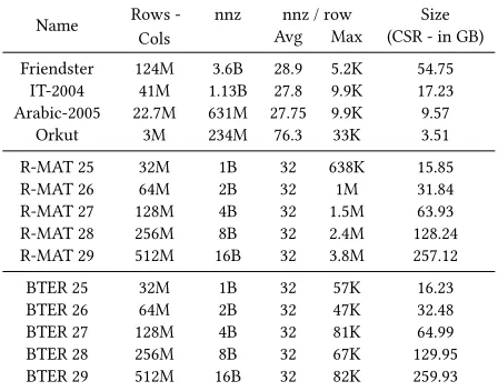
We study the performance of SpMV using graph matrices, includ-ing real-world graphs from the University of Florida Sparse Matrix Collection [6] and the Stanford Large Network Dataset Collec-tion [10], in addiCollec-tion to synthetic matrices of various sizes gener-ated using two well-known graph generators, R-MAT and BTER. R-MAT graphs are generated with the following parameters:a=
0.57,b = 0.19,c = 0.19,d = 0.05,e f = 16. For BTER we
com-puteα andδusing the reference code [9]; the other parameters arecmax = 0.5,дcc = 0.15,e f = 16. Both generators produce
Name Rows -Cols
nnz nnz / row Size Avg Max (CSR - in GB)
Friendster 124M 3.6B 28.9 5.2K 54.75 IT-2004 41M 1.13B 27.8 9.9K 17.23 Arabic-2005 22.7M 631M 27.75 9.9K 9.57
Orkut 3M 234M 76.3 33K 3.51
R-MAT 25 32M 1B 32 638K 15.85
R-MAT 26 64M 2B 32 1M 31.84
R-MAT 27 128M 4B 32 1.5M 63.93
R-MAT 28 256M 8B 32 2.4M 128.24 R-MAT 29 512M 16B 32 3.8M 257.12
BTER 25 32M 1B 32 57K 16.23
BTER 26 64M 2B 32 47K 32.48
BTER 27 128M 4B 32 81K 64.99
BTER 28 256M 8B 32 67K 129.95
BTER 29 512M 16B 32 82K 259.93
Table 2: Test matrices used in performance evaluation.
Performance results are measured on the architecture previously described in Section 2. We compare the streaming implementation against the CPU algorithms described in [4], because they represent the current state of the art for large-scale graph-based SpMV in shared memory systems.
The CPU-based SpMV implementation is written in standard C99 and is compiled with gcc v4.8.5 using –O3 optimization. SpMV kernels are optimized using inline assembly. The presented per-formance results are calculated by averaging the results of five executions, each performing ten SpMV iterations.
Two different algorithms are presented in [4]: a blocking algo-rithm and a binning algoalgo-rithm, with the latter outperforming the former. Compared to the previously published results, however, this server is equipped with 2 POWER 8 processors (instead of 8), thus has less memory bandwidth and a less prominent NUMA effect. Graphs are also smaller because of the lower amount of total system memory (512 GB instead of 2 TB). As a result, on this architecture, the Blocking algorithm outperforms the Binning one (confirming that the architecture plays a very important role in determining the best SpMV algorithm), so in this paper we only present results for the Blocking algorithm. We use sparse blocks of 64k×64k ele-ments, and present the best result among 2 and 4 threads/core. Our GPU-based SpMV implementation is written in standard C++11 and is compiled with gcc v4.8.5 using –O3 optimization. SpMV ker-nels are offloaded usingcusparse, while memory transfers exploit CUDA’s memory copy primitives. We exploit CUDA streams to allow transfers and computations to run concurrently on the GPU. According to the results in Section 2, to improve performance and allow asynchronous transfers, matrix blocks are allocated using pinned memory. The measured execution time includes the copy of the result back on the host memory. In this case, because of the high consistency and stability of GPU kernels, results are calcu-lated by averaging the results of 3 executions, each performing a single SpMV. In the GPU experiments we empirically found out that a good trade-off between streaming effect, amount of data transferred, and computation balancing can be achieved by using a
fixed number of 14 blocks per partition∗. Therefore, all the results presented in this section use GPU partitions with 14 blocks.
GFlop/s are always computed by considering the two floating point operations per element (nnz) of the original matrix.
Both the CPU and the GPU implementations use scrambling to improve load balancing of the graphs.
4.2
Performance Comparison
We begin our experiments by comparing the performance of the streaming GPU implementation against the current state of the art for large-scale graphs on shared-memory systems [4].
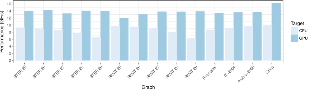
The CPU implementation peaks at∼10GF/s, with performance slowly degrading as the size of the matrix increases. Our streaming GPU implementation shows much better results. Using R-MAT, the performance starts at∼11.89GF/sand grows up to∼13.83GF/s. This represents an improvement over the CPU between 23% and 120%, depending on the matrix. With BTER graphs, the performance is even more steady, ranging from∼13.22GF/sto∼14.15GF/s, offering an improvement over the CPU between 51% and 115%. Similar results are confirmed with real-world graphs, with the CPU version, again, achieving results between∼8.5GF/sand 9.88GF/s, and the GPU version is always above∼13.4GF/s, and a maximum with Orkut of∼16.20GF/s, resulting in an improvement between 41% and 64%.
These numbers are not as high as the ones we modeled in the previous section using only transfer sizes and bandwidths. This means there are other overheads we did not consider in the model. In particular, we verified that the use of graph matrices puts an in-creased burden on the GPU’s threading and memory system which can cause imbalance among GPUs even with a fixed number of nnz per partition. As a result, in some cases, the computation can become more expensive than the communication—introducing an overhead we did not account for in the model. GPUs stream data independently, therefore we can still achieve a good computation balancing if this overhead is evenly spread among blocks of differ-ent GPUs. Unfortunately, there are cases (especially with smaller matrices such as the R-MAT 25) where the overhead is mostly paid by a single GPU, causing imbalance and therefore introducing ad-ditional overhead. We show this effect in Table 3 by presenting the performance of each individual GPU in the R-MAT 25 experiments. We can clearly see that, although the number of elements is bal-anced, the performance of GPU 2 is lower. An additional study with NVIDIA’s profiler verified that this is caused by longer execution times in thecusparseSpMV kernel.
Nevertheless, the final results show our streaming implemen-tation offering an average improvement of 62% over the previous state of the art for large-scale graphs.
4.3
Scalability Study
We conclude our experiments by evaluating both strong and weak scaling of our algorithms by using a variable number of GPUs.
For the strong scaling study, we selected a specific matrix, an R-MAT 27, and varied the number of GPUs in the test from 1 to 4. For the weak scaling, we kept the work per GPU fixed by increasing
0 2 4 6 8 10 12 14 16
BTER 25 BTER 26 BTER 27 BTER 28 BTER 29 RMA
T 25 RMA
T 26 RMA
T 27 RMA
T 28 RMA
T 29
Friendster IT−2004 Arabic−2005
Orkut
Graph
P
erf
or
mance (GF/s)
Target
CPU
GPU
Figure 5: Performance comparison of CPU and streaming GPU performance on Real World and Synthetic Graphs.
●
●
●
●
1.0 1.5 2.0
1 2 3 4
GPUS
Ex
ecution Time (s)
(a) Strong Scaling.
●
●
●
4 6 8 10 12 14
1 2 3 4
GPUS
P
erf
or
mance (GF/s)
(b) Weak Scaling.
Figure 6: Scaling on R-MAT.
GPU nnz Time Performance
Number (s) (GFlop/s)
GPU 0 261805091 0.150657 3.475516 GPU 1 261802582 0.150595 3.476903 GPU 2 261799623 0.175415 2.984909 GPU 3 261799470 0.149405 3.504558 Aggregate 1047206766 0.175441 11.937977
Table 3: Execution Profile for R-MAT 25.
the number of nnz of the matrix. Due to limitations in our graph generators, we can only grow the graph by a factor of 2†. Therefore, we gather points for 1,2, and 4 GPUs. We start with an R-MAT scale 25 on a single GPU and end with an R-MAT scale 27 on 4 GPUs.
The results in Figure 6 show a good profile in both cases, high-lighting the good scaling properties of our streaming implementa-tions. It should be noted, however, that because of the partitioning mechanism, we do not expect a perfect scaling. For each partition we have to re-transfer the whole input vector, therefore increasing
†We could change the edge factor but this would significantly change the structure
of the matrix, making the comparison unfair.
the amount of data to be transferred. In both cases, the 2-GPU speedup is approximately 1.8×, while the 4-GPU speedup reaches about 3.5×the performance of a single GPU.
5
RELATED WORK
The importance of SpMV as a kernel for graph processing and many other fields of engineering and science has lead to a broad variety of studies. A few examples with focus on CPU-based SpMV can be found in [8], [13] and [14].
Over the past years, the offload of processing to accelerators like GPUs, FPGAs, or many-core co-processors became more and more important and popular. This created a revived interest in SpMV, mostly because of its irregular pattern and low arithmetic inten-sity, that led to a large variety of new matrix formats specifically targeting GPUs. Among the most relevant works are [5], [7], [11] and [15].
Reference Max Size Architecture
Best R-MAT Perf. [GFlops/s] (Parameters)
Ashari
et al. [2] 298M nnz GPU N/A
Tang
et al. [12] 29M nnz
Many-core Coprocessor
∼7 (S 18, EF 32)
Boman
et al. [3] 1.6B nnz
CPU (Cluster)
256 Nodes 64.95 (S 26, EF 9)
Buono
et al. [4] 68B nnz
CPU
(Shared Mem.) 51.51 (S 26, EF 32) Our
Approach 17B nnz GPU (streaming) 13.81 (S 29, EF 32)
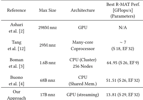
Table 4: State of the art results in the literature for graph-oriented SpMV algorithm. For synthetic graphs (R-MAT and BTER), S is the graph scale and EF the edge factor. Note that the results in [4] were obtained on a high-end Power SMP system, with8×the memory bandwidth of the system used in this paper.
Another example of GPU-optimized graph kernels can be found in [2]. The authors optimize the load balancing, with less focus on the amount and patterns of data that are accessed by the GPU. Their work uses binning techniques on top of standard CSR (called ACSR) to reduce the matrix pre-processing overheads and also allow for processing of dynamic graphs.
Tang et al. [12] utilize a many-core co-processor to run graph-specific SpMV. Similar to [2], they focus on load balancing and efficient use of the accelerator. Their approach includes a perfor-mance tuning guide to adjust the partitioning to different non-zero distributions of the matrix data (scale-free matrices).
Each of these approaches assumes that the entire matrix is small enough to fit inside the GPU memory, therefore limiting the size of the problem to a few GB. To the best of our knowledge, [4] is the first paper to introduce the concept of very large SpMV kernels for data analytics on shared memory systems.
In [4], a novel algorithm for CPU-based SpMV is presented, enabling the computation of matrix sizes of an order of magnitude larger than the ones previously analyzed, even in cluster-oriented papers like [16] and [3].
With this paper, we tackle very large matrices by solving prob-lems of two orders of magnitude larger than the current state of the art on GPUs, as shown in Table 4. To the best of our knowledge, we are the first to propose a streaming approach with larger matrices that can reside on the host memory.
6
CONCLUSION
In this paper we study the performance impact of NVLink on SpMV, a core example of a graph analytics kernel, and we show how NVLink enables computation on a much larger scale than previ-ously possible. By leveraging NVLink, our experiments show that,
not only the problem scale can be increased, but, on the same sys-tem, the streaming version of SpMV that uses NVLink achieves approximately 50% better performance than the state-of-the-art CPU implementation. Given the ubiquitous nature of SpMV, and its sharing of common traits with other analytics kernels, we be-lieve that NVLink can also benefit a variety of other data analytics problems.
REFERENCES
[1] Pham Nguyen Quang Anh, Rui Fan, and Yonggang Wen. 2015. Reducing Vector I/O for Faster GPU Sparse Matrix-Vector Multiplication. InParallel and Dis-tributed Processing Symposium (IPDPS), 2015 IEEE International. 1043–1052.DOI:
http://dx.doi.org/10.1109/IPDPS.2015.100
[2] Arash Ashari, Naser Sedaghati, John Eisenlohr, Srinivasan Parthasarathy, and P. Sadayappan. 2014. Fast Sparse Matrix-vector Multiplication on GPUs for Graph Applications. InProceedings of the International Conference for High Performance Computing, Networking, Storage and Analysis (SC ’14). IEEE Press, Piscataway, NJ, USA, 781–792.DOI:http://dx.doi.org/10.1109/SC.2014.69
[3] Erik G. Boman, Karen D. Devine, and Sivasankaran Rajamanickam. 2013. Scalable Matrix Computations on Large Scale-free Graphs Using 2D Graph Partitioning. InProceedings of the International Conference on High Performance Computing, Networking, Storage and Analysis (SC ’13). ACM, New York, NY, USA, Article 50, 12 pages.DOI:http://dx.doi.org/10.1145/2503210.2503293
[4] Daniele Buono, Fabrizio Petrini, Fabio Checconi, Xing Liu, Xinyu Que, Chris Long, and Tai-Ching Tuan. 2016. Optimizing Sparse Matrix-Vector Multiplication for Large-Scale Data Analytics. InProceedings of the 2016 International Conference on Supercomputing (ICS ’16). ACM, New York, NY, USA, Article 37, 12 pages.
DOI:http://dx.doi.org/10.1145/2925426.2926278
[5] J.W. Choi, A. Singh, and R.W. Vuduc. 2010. Model-driven autotuning of sparse matrix-vector multiply on GPUs. InACM SIGPLAN Notices, Vol. 45. ACM, 115– 126.
[6] T.A. Davis. 1994. The University of Florida sparse matrix collection. InNA digest. Citeseer.
[7] Joseph L. Greathouse and Mayank Daga. 2014. Efficient Sparse Matrix-vector Multiplication on GPUs Using the CSR Storage Format. InProceedings of the International Conference for High Performance Computing, Networking, Storage and Analysis (SC ’14). IEEE Press, Piscataway, NJ, USA, 769–780. DOI:http: //dx.doi.org/10.1109/SC.2014.68
[8] E.J. Im, K. Yelick, and R. Vuduc. 2004. SPARSITY: Optimization framework for sparse matrix kernels.Intl J. High Perf. Comput. Appl.18 (2004), 135–158. [9] Tamara G. Kolda, Ali Pinar, Todd Plantenga, and C. Seshadhri. 2014. A Scalable
Generative Graph Model with Community Structure.SIAM Journal on Scientific Computing36, 5 (September 2014), C424–C452.DOI:http://dx.doi.org/10.1137/ 130914218
[10] Jure Leskovec and Andrej Krevl. 2014. SNAP Datasets: Stanford Large Network Dataset Collection. http://snap.stanford.edu/data. (June 2014).
[11] Xing Liu, Mikhail Smelyanskiy, Edmond Chow, and Pradeep Dubey. 2013. Effi-cient Sparse Matrix-vector Multiplication on x86-based Many-core Processors. InProceedings of the 27th International ACM Conference on International Con-ference on Supercomputing (ICS ’13). ACM, New York, NY, USA, 273–282.DOI:
http://dx.doi.org/10.1145/2464996.2465013
[12] Wai Teng Tang, Ruizhe Zhao, Mian Lu, Yun Liang, Huynh Phung Huynh, Xibai Li, and Rick Siow Mong Goh. 2015. Optimizing and Auto-tuning Scale-free Sparse Matrix-vector Multiplication on Intel Xeon Phi. InProceedings of the 13th Annual IEEE/ACM International Symposium on Code Generation and Optimization (CGO ’15). IEEE Computer Society, Washington, DC, USA, 136–145. http://dl. acm.org/citation.cfm?id=2738600.2738618
[13] Richard Wilson Vuduc. 2003. Automatic performance tuning of sparse matrix kernels. Ph.D. Dissertation. Univ. of California, Berkeley.
[14] Samuel Williams, Leonid Oliker, Richard Vuduc, John Shalf, Katherine Yelick, and James Demmel. 2007. Optimization of sparse matrix-vector multiplication on emerging multicore platforms. InProc. ACM/IEEE Conf. Supercomputing (SC ’07). ACM, New York, NY, USA, 38:1–38:12.DOI:http://dx.doi.org/10.1145/1362622. 1362674
[15] Shengen Yan, Chao Li, Yunquan Zhang, and Huiyang Zhou. 2014. yaSpMV: Yet Another SpMV Framework on GPUs. InProceedings of the 19th ACM SIGPLAN Symposium on Principles and Practice of Parallel Programming (PPoPP ’14). ACM, New York, NY, USA, 107–118.DOI:http://dx.doi.org/10.1145/2555243.2555255 [16] Andy Yoo, Allison H. Baker, Roger Pearce, and Van Emden Henson. 2011. A