R E S E A R C H A R T I C L E
Open Access
Robust model reduction by
L
1
-norm
minimization and approximation via
dictionaries: application to nonlinear
hyperbolic problems
Rémi Abgrall
1, David Amsallem
2and Roxana Crisovan
3**Correspondence:
3Institut für Mathematik,
Universität Zürich, Winterthurerstrasse 190, CH-8057 Zürich, Switzerland Full list of author information is available at the end of the article
Abstract
We propose a novel model reduction approach for the approximation of non linear hyperbolic equations in the scalar and the system cases. The approach relies on an offline computation of a dictionary of solutions together with an onlineL1- norm minimization of the residual. It is shown why this is a natural framework for hyperbolic problems and tested on nonlinear problems such as Burgers’ equation and the one-dimensional Euler equations involving shocks and discontinuities. Efficient algorithms are presented for the computation of theL1-norm minimizer, both in the cases of linear and nonlinear residuals. Results indicate that the method has the potential of being accurate when involving only very few modes, generating physically acceptable, oscillation-free, solutions.
Keywords: Model reduction, Dictionaries,L1-norm residual minimization
Background
Many engineering applications require the ability to simulate the behavior of a physical system in real-time. This requirement holds in particular when a full parametric explo-ration of the behavior of the system is sought. In aerodynamics, such an exploexplo-ration can be done to compute the flow around an aircraft for varying boundary conditions or to design its shape to maximize lift and minimize drag. Uncertainty quantification also requires a large number of simulations with varying parameters in order to propagate chaos by means of a Monte-Carlo method or calibrating input parameters by a Markov chain technique. A third important application is flow control.
When such a large number of simulations is required, the cost of one simulation is critical to the application at hand. This cost can be lowered by using sophisticated computer science techniques such as parallelization but such techniques are usually not enough to allow full parametric exploration, especially when computational resources are limited.
Alternatively, model reduction techniques can alleviate the cost of such repeated simula-tions with limited computational resources [1–4]. Model reduction is directly based on the underlying high-dimensional model (HDM) that results from a standard finite element,
©2016 Abgrall et al. This article is distributed under the terms of the Creative Commons Attribution 4.0 International License (http://creativecommons.org/licenses/by/4.0/), which permits unrestricted use, distribution, and reproduction in any medium, provided you give appropriate credit to the original author(s) and the source, provide a link to the Creative Commons license, and indicate if changes were made.
finite volume or finite differences formulation. In the present paper, partial differential equations (PDE) of the following type are considered:
∂U
∂t +L(U)=0 x∈, t∈[0, T] B(U)=g x∈∂, t∈[0, T] U(x, t=0)=U0(x) x∈
(1)
Lis a differential operator (for example the Laplacian or the divergence of a flux), and Ba boundary operator. In this paper, we are particularly interested in the case where the solutionU(x, t) ∈ Rp is a scalar or a vector andLis the divergence of a fluxF. Three examples will be considered by increasing the order of complexity:
• Burgers’ equation for whichU=uis scalar:
– Its unsteady version,
∂u
∂t +
∂ ∂x
1 2u
2
=0, u(x,0)=u0(x)
with periodic boundary conditions
– It steady version with weak Dirichlet boundary conditions
• The one-dimensional compressible Euler equations for which
U =(ρ,ρu, E), F(U)=ρu,ρu2+p, u(E+p)
and the perfect gas equation of state holds:
p=(γ −1)
E− 1 2ρu
2
.
ρdenotes the density,uthe velocity,pthe pressure andEthe energy. • An example of a steady flow through a nozzle.
After discretization in space, the solution is denoted as u(t) ∈ RNp. The PDE is here parametrized by a parameter vectorμ∈ Rmthat allows changes in the operatorL, the
boundary operatorBor the initial conditions. For simplicity and without loss of generality, this parametric dependency will be omitted in the next paragraphs.
Instead of allowing any value of the solution degrees of freedomu, model reduction however restricts the solution to be contained in a subspace of the underlying high-dimensional space. This subspace is determined by an optimized reduced basis that is determined in a training phase. Thus, a large number of degrees of freedom (say millions) are represented by only a few number of coefficients in the representation of the full solution in terms of the reduced basis vectors, leading to important computational savings. Two important questions arise at this point: (1) how can an optimal reduced basis be constructed? and (2) how can the evolution of the reduced coefficients be computed in a stable fashion?
A popular method for choosing an “optimal” basis is Proper Orthogonal Decomposition (POD), first introduced as a tool for the analysis of flows by Lumley [5] and then extended and popularized by Sirovich [6]. The idea behind POD is to collect a few snapshots of the solution and then compute the best approximation of these snapshots in terms of a small number of reduced basis vectors. Mathematically speaking, ifui(tl)∈Rpdenotes the value
constructsMorthogonal functionsφ ∈L2(Rd)psuch that the following functional is
minimized:
J(φ1,. . .,φM)=
Nt
l=1
Np
i=1
ui(tl)−
M
=1
u(tl),φφi 2
2
, (2)
whereφi ∈Rpdenotes the value ofφatxi. · denotes here the Euclidean norm inRp,
and · , · is theL2scalar product. A minimum of the functionalJ can be analytically computed by Singular Value Decomposition and the reduced basis vectorsφare the left singular vectors of the snapshots matrix
S= ⎛ ⎜ ⎜ ⎝
u1(t1) . . . u1(tNt)
..
. ... ... uN(t1) . . . uN(tNt)
⎞ ⎟ ⎟ ⎠.
Defining by{λ}Nt
l=1the positive eigenvalues ofSTSsorted decreasingly, the error
associ-ated with the minimum of the functional is
J(φ1,. . .,φM)=
Nt
=M+1
λ. (3)
In the continuous case, the functionsφ(x)∈Rp, are the solution of Fredholm
alterna-tive
R(x,x
)φ
(x)dx=λφ(x), for allx∈, (4)
whereR(x,x)=u(x)u(x)T.
In both the discrete and continuous cases, the basis dimensionMis depending on how fast is the decay of the eigenvalues λ. Given a tolerance 1,Mis selected as the smallest dimension such that the following relative truncation error is smaller than ,
J(φ1,. . .,φM) Nt
l=1
Np
i=1 ui(tl) 22
= Nt
=M+1λ
Nt
=1λ
. (5)
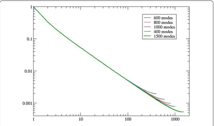
In general, one expects the eigenvaluesλto decrease very rapidly to 0. This allows, when this assumption is true, to consider only the most energetic modes in the decomposition. Unfortunately, it is not always the case that the eigenvaluesλare rapidly converging to zero. This is demonstrated by the following simple counter example for which a simple scalar advection problem defined on=[0,1[ is considered:
∂u
∂t +
∂u
∂x =0 (6a)
with the boundary condition
u(0, t)=1 (6b)
and the initial condition
u(x,0)=0. (6c)
The solution is given by a traveling discontinuity
u(x, t)=
1 ifx≤min(t,1) 0 otherwise.
Considering grids xi = i/N, i = 0,. . ., N for varying number of grid pointsN and
constructed numerically. For each grid size N, the eigenvaluesλ(N) are reported in Fig.1. One can observe that the ratioλ(N)/λ1(N) behaves like 1/k. This illustrates that
it is not possible to select only a few dominant modes, due to the slow decay of the POD eigenvalues. This example also illustrates why most of the work on model reduction has been focused on regular problems, and for fluids, on incompressible flows, see e.g. among many others [7–9]. For compressible (but regular) flows, one of the early work is [10], then one may mention [11] for compressible turbulent flows and [3,12,13] for the case of linearized compressible inviscid flows.
Concerning compressible fluids, there is another difficulty. In problem (4), one needs a norm. In the case of incompressible flows, a natural norm is related to the kinetic energy. For compressible materials, however, one needs to take into account the density, velocity and the energy, i.e. the thermodynamics. A simpleL2-norm cannot be used because one cannot combine in a quadratic manner these variables, for dimensional reasons. Only a non-dimensionalization of the variables can alleviate the dimensionality issue [11,12].
The natural equivalent of theL2-norm is however related to the entropy, which is not quadratic: if a minimization problem can be set up, its solution is non trivial. These arguments were raised in [10], and an energy-based norm was developed in [13] for linearized compressible flows.
To circumvent those issues, an approach based on a dictionary of solutions [14] is developed in this work as an alternative to using a truncated reduced basis based on POD. The elements of this dictionary are solutionsu(tl;μj) computed for varying values of time tl and parameterμj ∈ Rm. Selecting appropriate parameter samplesμj ∈ D ⊂ Rm is
a crucial step that can affect the accuracy of the reduced-order model in the parameter domain. Greedy sampling procedures have been developed when error estimates are known [7,9,15–17]. In this work, we do not elaborate much on this, we are more focused on showing that such a method can actually work. The strategy to look for the “best”μin this context will be the topic of further research.
Fig. 1 In log–log coordinate, plot of the ratio of POD eigenvalues log(λk(N)/λ1(N)) for
In addition to choosing an appropriate dictionaryD, selecting an approach for comput-ing a reduced solution based on that dictionary is also crucial. For self-adjoint systems, Galerkin projection is a natural approach but it there is no motivation for using Galerkin projection for nonlinear compressible flows. Instead, strategies based on the minimization of the residual arising from the reduced approximation have been successfully developed for compressible flows in [1,2,11]. These approaches rely on a minimization of the residual in theL2sense. In the present work, this minimization problem is extended to the more general minimization using aLq-norm, with emphasis onq=1. For nonlinear systems, an additional step, hyper-reduction, is required to ensure an efficient solution of the reduced system [11,18]. Hyper-reduction is not considered in this work but will be the subject of follow-up work.
Methods
This section is organized as follows. Motivations for using theL1norm in the case of hyper-bolic systems are presented first. We show thatq=1 is very closely linked to the concept of weak solutions of hyperbolic problems. Then, the proposed model reduction approach is developed in both the steady and unsteady cases. Finally, the proposed procedure is applied to the model reduction of several steady and unsteady systems and conclusions are given in the end.
Motivation for theL1-norm
In solving minimization problems, it is quite usual to minimize some residual with respect to theLqnorm for suitableq. The choiceq = 2 is very common because it amounts to minimize in some least square sense and many efficient algorithms are available. In the case of hyperbolic problems, as we are concerned with here, this is still a convenient choice (after proper adimensionalization as mentioned above), but it might not be the most natural one. For example in [19,20] it is shown at least experimentally, that the numerical solution has an excellent non oscillatory behavior, without doing explicitly anything but to minimize theL1norm of the PDE residual. In fact, this observation was
our original motivation for choosing theL1norm, since we are interested in keeping the non oscillatory nature of the solution. In this section, we further justify the choice of the L1norm applied to the residual, and show that it is closely related to the weak formulation of the problem. The discussion is here formal.
Let us consider the problem
∂U
∂t + divF(U)=0 (7)
defined on ⊂Rd,t > 0. The steady problem can be done in the same exact manner.
We assume that the solutionUbelongs toRp, so thatF=(F1,. . ., Fp). The weak form of
this is: for anyϕ∈C1()pand with compact support, we have:
ϕ(x, t)
∂
U
∂t + divF(U)
dx=0.
Integrating by parts, yields
∂ϕ ∂tUdx+
If we restrict ourselves to the set of test functions ϕ∈C1()p,||ϕ||∞≤1, U is a solution if:
sup {ϕ∈[C1()]p,||ϕ||
∞≤1}
∂ϕ ∂tUdx+
∇ϕ·F(U)dx
=0.
Let us now recall the definition of the total variation
TV(g)= sup
ϕ∈C01(Rn)∩L∞(Rn),||ϕ||∞≤1
Rn∇ϕ
(x)·g(x)dx
,
and the definition of the bounded variation of a functiong ∈L1(Rn):
BV(Rn)=g ∈L1(Rn) : TV(g)<∞.
We see that if in additiong ∈C1(Rn),TV(g)=Rn||∇g||dx= ||∇g||L1(Rn).
Thanks to this definition, we see that if we define the space-time fluxF =(U, F),Uis a weak solution if and only if the total variation ofFvanishes,TVF)=0.
Before going further, let us mention the following classical result that will be useful. Consider {xi}i∈Z a strictly increasing sequence in R, we definexi+1/2 = xi+2xi+1. We
assume thatR= ∪i∈Z[xi−1/2, xi+1/2[ and considergdefined by: for anyi∈Z,
g(x)=gi ifx∈[xi−1/2, xi+1/2[,
we see that
TV(g)=
i∈Z
|gi+1−gi|.
Now, instead of having the exact solution, but some approximation procedure that enables, fromun≈U(. , tn), to computeun+1≈U(. , tn+1), sayL(un,un+1).
For instance, assume that we have a finite volume method andd=1: for any grid point i∈ {1,. . ., N},
Lun,un+1
i=x
un+1
i −uni
+tfi+1/2(un)−fi−1/2(un)
.
A way to evaluateun+1is to minimize the total variation, i.e.
TV(L)=
i∈I
xuni+1−uni+tfi+1/2(un)−fi−1/2(un),
un+1= argmin
vpiecewise constant
i∈I
xvi−uni
+tfi+1/2(un)−fi−1/2(un).
Clearly, ifIis equal to the set of grid points, the solution is given by
un+1
i =uin− t
x
fi+1/2(un)−fi−1/2(un)
and nothing new is gained.
WhenIis not equal to the set of degrees of freedom, then something new happens. We expect precisely to exploit this idea, or ideas related to this.
Formulation
High-dimensional model
Without loss of generality, the case of the classical finite volume method is considered to define the High Dimensional Model (HDM). A computational domain ⊂ Rd is considered, and in most of this paper,⊂R, that isd =1. Starting from a subdivision · · ·<xj <xj+1<· · ·, we construct control volumesKj=[xj−1/2, xj+1/2[,j∈Zwhere
xj+1/2=
xj+xj+1
2 .
A finite volume semi-discrete formulation of (1) writes |Kj|
duj
dt +fj+1/2(u)−fj−1/2(u)=0 (8a) wherefj+1/2is a consistent numerical flux. In each applications, we consider Roe’s
formu-lation and a first order scheme. We assume either compactly supported initial conditions or initial conditions with periodicity
uj(t=0)≈
1 |Kj|
Kj
U0(x)dx. (8b)
In (8a),ujstands for an approximation of the average of the solution in the cellKj,
uj(t)≈
1 |Kj|
Kj
U(x, t)dx.
The time stepping is done in a standard way, for instant by Euler time stepping.
Model reduction by residual minimization over a dictionary Steady problems
Two approaches are available to solve a steady state associated with problem (1). The first one is to use a homotopy approach with pseudo-time stepping, resulting in the solution of an unsteady problem which limit solution is the desired steady state. The procedure described in Sect. “Unsteady problems” can be, in principle applied to this case. The second approach is by a direct solution of the steady-state problem. The discretized steady-state problem writes
r(u(μ),μ)=0
wherer(·,·) is usually a nonlinear function of its arguments, referred to as the residual. This set of nonlinear equations is typically solved by Newton-Raphson’s method. This second approach is followed in this work for steady problems.
The parameter vectorμ∈ P ⊂ Rmcan, for instance, parametrize the boundary con-ditions associated with the steady-state problem. The parametric domain of interestPis assumed here to be a bounded set ofRm.
The solution manifoldM=u(μ) s.tμ∈P ⊂Rmis assumed to be of small dimen-sion. This manifoldMbelongs toL∞(Rd)∩BV(Rd), and thus can be locally described by some mappingθ :P →L∞(Rd)∩BV(Rd). To approximate this mapping, we consider a family ofrparameters inP,{μ}r=1, and compute the associated solutionsu(μ)r=1 of (8).
The steady-stateu(μ) is then approximated as a linear combination of the precomputed dictionary elementsDas
u(μ)≈
r
=1
For a new value of the parametersμ∈P, the reduced coordinatesα(μ)r=1are then computed as the solution of the minimization problem
α(μ) :=(α1(μ),. . .,αr(μ))= argmin β=(β1,...,βr)
J
r
r
=1
βu(μl),μ
,β
. (10)
In this paper we consider forJ theL1-normJ(r,β)= r1or its regularized variant,
J(r,β)= r1+ηβ1withη >0.
In order to minimizeJ whenris a linear function ofβ, the Linear Programming (LP) approach is considered, involving the solution of an optimization problem with 2m+r variables and 3mconstraints.
Whenris a nonlinear function ofβ, a Gauss-Newton-like procedure can be used in combination with the LP approach. Unicity of the solution can be guaranteed by setting the regularization termη >0. That’s why we are not doing the linear example.
Remark • Decreasing the dimensionality of the solution space fromNtoris not enough to gain computational speedup when the system to be solved is nonlinear. An addi-tional level of approximation, hyper-reduction, is necessary.
• A careful selection of the sample parameter samplesμr=1is necessary in order to generate a reduced-order model that is accurate in the entire parameter domain P. Greedy sampling techniques, associated with a posteriori error estimates, have been successfully used to construct reduced models that are robust and accurate in a parameter domainP. These techniques are not considered in this paper but will also be the focus of future work.
Unsteady problems
For simplicity, in the remainder of this section, we assume that only the initial condition u0(μ) depends on a parameter vectorμ∈P ⊂Rm. Again, the family of solutionsu(μ) of
the Cauchy problem (8) is then conjectured to belong to a low dimensional manifoldM when the initial condition is parametrized in (8b).
To approximate this mapping, we consider a family of r parameters inP, {μ}r=1, and compute the associated solutions of (8) for respective initial conditionsu0(μ),= 1,. . ., r.
Once these solutions are computed, we propose to approximate, for any parameter
μ∈Pthe solution{un(μ)}Nt
n=0associated with an initial conditionu0(μ) by approximating
it as
un(μ)= r
=1
αn(μ)un(μ )
with the following procedure:
1. Initialization: determine the reduced coefficients{α0(μ)}r=1as:
α0(μ) :=α0
1(μ),. . .,α0r(μ)
= argmin
β=(β1,...,βr)
J
r
=1
βu0(μ
),β
,
2. Assume thatαn(μ) = (αn
1(μ),. . .,αrn(μ)) is known, determineαn+1 = (α1n+1,. . .,
αn+1
r ) such that:
αn+1(μ)= argmin β=(β1,...,βr)
J
r
=1
βun+1(μ)−wn(μ)− t
x
f1/2(wn)−f−1/2(wn)
,β
where
wn(μ)= r
=1
αn
(μ)un(μ).
We see that the second step can be written as: findαn+1(μ) that minimizes
JAn+1αn+1−bn:=JAn+1αn+1−bn,αn+1
where the matrixAn+1can be written by blocks as
An+1=
⎛ ⎜ ⎜ ⎝
un+1
1 (μ1) . . . un1+1(μr)
..
. ... ... un+1
N (μ1) . . . unN+1(μr) ⎞ ⎟ ⎟
⎠ (11)
andbndepends on known data.
A few immediate remarks can be made.
Remark • In the case of a linear flux, Problem (1) is linear. IfStis the mapping between
the initial conditionu0and the solution at timet, we haveSt(u+v)=St(u)+St(v).
This means the exact solution of the Cauchy problem withU0 = α0U0(μ) is
St(U0)= α0St(U(μ,0)). In the case of a linear scheme, minimizing the
func-tionalJshould result inαn=α0for anyn≥0.
• In the case of an explicit background scheme, the choice of the numerical flux, how high order is reached, and the choice of time stepping has no influence on the overall procedure: any sub-time step would be treated similarly. In this paper, we have chosen a first order method with Euler time stepping in the case of unsteady problem. • In the case of an implicit scheme, a Newton-like procedure can be applied to minimize
the functional as in [11]. At each time step, the procedure is then identical as in the steady case described above.
Results and discussion
Model reduction of unsteady problems
Unsteady Burgers’ equation
We consider here the system (7) in =[0,2π] with periodic boundary conditions and the initial conditions parameterized by
u0(x;μ)=μsin(2x)+0.1,
whereμ∈[0,1]. In this setting, the solution develops a shock that moves with the velocity
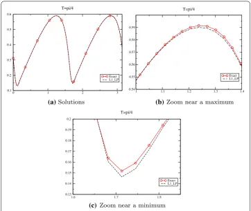
σμ=0.55μ. A dictionaryDis constructed by sampling the parameters{0,0.2,0.4,0.6,1.0} (r = 5) and the solution sought for the predictive caseμ = 0.5. A shock appears at t =1. We display the solutions obtained byL1-norm by LP minimization procedure for t= π4 <1,t= π2 andt=πin Figs.2,3.
3 2
1 0
0.1 0.2 0.3 0.4 0.5 0.6
Exact L1_LP T=pi/4
(a) (b)
(c)
1 1.1 1.2 1.3 1.4
0.54 0.55 0.56 0.57 0.58 0.59
Exact L1_LP T=pi/4
1.6 1.7 1.8
0.13 0.14 0.15 0.16 0.17 0.18 0.19 0.2
Exact L1_LP T=pi/4
Solutions Zoom near a maximum
Zoom near a minimum
Fig. 2 Unsteady Burgers’ equation: predicted solutions at target parameterμ=0.5 att=π4
3 2
1 0
0.1 0.2 0.3 0.4 0.5 0.6
Exact L1_LP
T=pi/2
(a)
3 2
1 0
0.2 0.3 0.4 0.5
Exact L1_LP
T=pi
(b)
Fig. 3 Unsteady Burgers’ equation: predicted solutions at target parameterμ=0.5 att=π2 (left) and t=π(right)
att =π. Nevertheless, theL1-norm-type solutions are within the bounds of the “exact” solution, and no large oscillation develops.
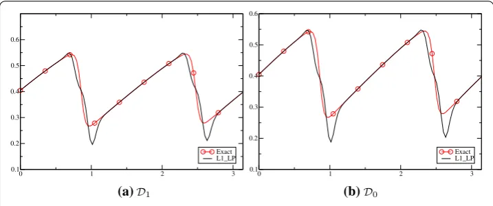
In a second set of numerical experiments, we consider the influence of the sam-pling parameter set included in the dictionary D. We consider two dictionariesD1 =
3 2 1 0 0.1 0.2 0.3 0.4 0.5 0.6 Exact L1_LP (a) 3 2 1 0 0.1 0.2 0.3 0.4 0.5 0.6 Exact L1_LP (b)
D1 D0
Fig. 4 Unsteady Burgers’ equation: predicted solutions at target parameterμ=0.5 att=πfor two dictionaries associated with two samples of the parameter domainP
μ=0.5. These choices amounts to selecting samples close to the target value 0.5 while
varying elements of the dictionary that are not close to 0.5 (see Fig.4).
We see that refining the dictionary has a positive influence as the target solution is much closer to the dictionary elements. This is confirmed by additional experiments where the samples ofμused to generate the dictionary where more numerous and closer to 0.5 (not reported here). TheL1-norm-type solutions are however unaffected by the presence of these “outliers” in the dictionary.
Euler equations
The one-dimensional Euler equations are considered on=[0,1]
∂ ∂t ⎛ ⎜ ⎝ ρ ρu E ⎞ ⎟ ⎠+ ∂∂ x ⎛ ⎜ ⎝ ρu
ρu2+p u(E+p)
⎞ ⎟
⎠=0, (12a)
for whichU =(ρ,ρu, E)Tand the pressure is given by
p=(γ −1)
E− 1 2ρu
2
(12b)
withγ =1.4.
This problem is parametrized by the initial conditions U0(x;μ). To define the
para-metrized initial conditions of the problem, the Lax and Sod cases are first introduced as follows.
The stateUSod(x) is defined by the primal physical quantities:
VSod(x)=
⎧ ⎪ ⎨ ⎪ ⎩
ρ=1 ifx≤0.5,0.125 otherwise, u=0.0
p=1.0 ifx≤0.5, 0.1 otherwise,
(12c)
andULax(x) defined by
VLax(x)=
⎧ ⎪ ⎨ ⎪ ⎩
ρ=0.445 ifx≤0.5,0.5 otherwise, u=0.698 ifx≤0.5, 0.0 otherwise, p=3.528 ifx≤0.5, 0.571 otherwise.
(12d)
solution has a very different behavior and the contact is much stronger. This is depicted in Fig.5where the two solutions are shown fort=0.16.
The initial condition are parametrized forμ∈[0,1] as
V0(x;μ)=μVSod(x)+(1−μ)VLax(x) (12e)
and the conservative initial variablesU0(x;μ) constructed fromV0(x;μ).
In the subsequent numerical experiments, two strategies are exploited to construct, from the dictionaryD, the approximationun(μ) of the solution at each time stepn:
• Either we reconstruct together the discretized density vectorsρ, momentumm=ρu and energyE, i.e. the state variable at timetnusing only one coefficient vectorαn=
(αn1,. . .,αrn)
un= ⎛ ⎜ ⎝
ρn
mn
En ⎞ ⎟
⎠≈
r
j=1
αn
jun(μj). (13)
Here the{αn
j}rj=1are obtained by minimizingJon the density components of the state
because the density enable to detect fans, contact discontinuities and shocks, con-trarily to pressure and velocity which are constant across contact waves. Doing so we expect to control better the numerical oscillations, if any, than with the other physical variables. Similar arguments could be applied with the other conserved variables as well.
• Alternatively, we reconstruct each conserved variable separately
ρn≈ r
j=1
αn
jρn(μj), mn≈ r
j=1
αn
jmn(μj), En≈ r
j=1
αn
jEn(μj). (14)
where the minimization procedures are doneindependentlyon each conserved vari-able.
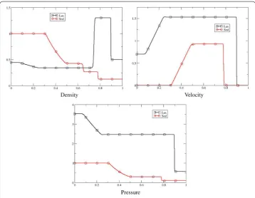
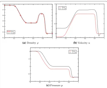
In order to test these approaches, the PDE is discretized by finite volumes using a dis-cretization resulting inNp=3000 dofs. The parameter rangeD= {0.0,0.2,0.4,0.5,0.8,1} is considered together with a targetμ=0.6. The results using the first strategy, see eq. (13), are displayed in Fig.6and those using the second strategy, see eq. (14), reported in Fig.7.
From both figures, we can see that the overall structure of the solutions is correct. Nevertheless, there are differences that can be highlighted. From Fig.6, we can observe that the density predictions, besides an undershoot at the shock, are well reproduced. However, we cannot recover correct values of the initial velocity (see left boundary), because there is no reason to believe that the coefficientα, evaluated from the density only, will also be correct for the momentum. A careful observation of the pressure plot also reveals the same behavior which is not satisfactory. For the same reason, if any other singlevariable is used for a global approximation of each conservative variables, there no reason why better qualitative results could be obtained.
0 0.2 0.4 0.6 0.8 1
0.2 0.3 0.4 0.5 0.6 0.7 0.8
Exact L1_LP
(a) (b)
(c)
0 0.2 0.4 0.6 0.8 1
0 0.5 1 1.5
Exact L1_LP
0 0.2 0.4 0.6 0.8 1
0 0.5 1 1.5
2 Exact
L1_LP
Densityρ Velocityu
Pressurep
0 0.2 0.4 0.6 0.8 1 0.2
0.3 0.4 0.5 0.6 0.7 0.8
Exact L1_LP
0 0.2 0.4 0.6 0.8 1
0 0.5 1 1.5 2
Exact L1_LP
0 0.2 0.4 0.6 0.8 1
0 0.5 1 1.5 2 2.5
Exact L1_LP
(a) (b)
(c)
Density ρ Velocityu
Pressurep
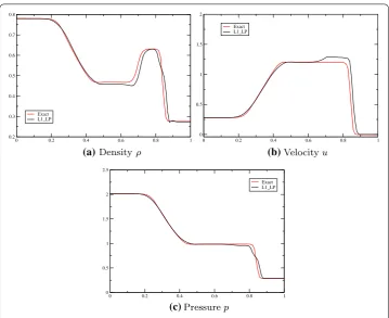
Fig. 7 One-dimensional Euler equations: predicted solutions with strategy (14) based on multiple expansions
This problem does not occur with the second strategy for the reconstruction (14): the correct initial values are recovered. We have some slight problems on the velocity, between the contact and the shock.
In order to obtain these results we have been faced to the following issue. Take the momentum, for example. For at least half of the mesh points, its value is 0, and for half of the points, its value is set to a constant. Hence, the matrixAused in the minimization procedure and built on the momentum dictionary has rank 2 only. The same is true for the other variables, and we are looking here forrcoefficients. Several approaches can be followed to address this issue. The first one relies on Gram-Schmidt orthogonalization of the solutions prior to their use as a basis for the solution. The second approach, followed here, consists into perturbing infinitesimally and randomly the matrices involved in the procedure, soAijis replaced byAij+εij. The distribution ofεij is uniform. This has the
effect of giving the maximum possible rank to the perturbed matrix. We have expressed that ijshould depend on the variable, we have chosen
εij= ijLref
whereLrefis the difference between the minimum and the maximum, over the dictionary,
of the considered variable. Choosing the sameεij for all variables, this has the effect of increasing the amplitude of the oscillations after then shock.
0 0.2 0.4 0.6 0.8 1 0
0.5 1 1.5 2
mu_1=1.3 mu_2=1.7 mu_3=1.4 mu_4=1.6 mu_5=1.8 mu=1.5(exact) L1
(a) (b)
0 0.2 0.4 0.6 0.8 1
0.2 0.4 0.6 0.8 1
mu_1=1.3 mu_2=1.7 mu_3=1.4 mu_4=1.6 mu_5=1.8 mu=1.5(exact) L1
Mach Density
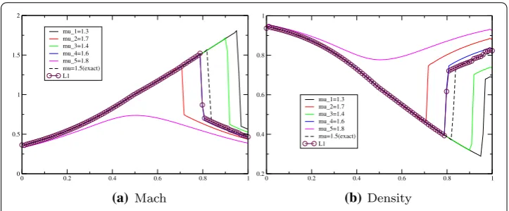
Fig. 8 Steady Nozzle flow: predicted solutions at target parameterμ=1.5
Model reduction of steady problems
Nozzle flow
To illustrate the ability of the reduced model, we consider the nozzle flow numerical experiment. The PDF is
∂F
∂x =S(U) where
U =(ρ,ρu, E)T, F(U)=Aρu, Aρu2+p, Au(E+p)T, S(U)=
0, p∂A
∂x,0 T
andAis the area of the nozzle flow. Depending on the boundary conditions, we can have a fully smooth flow or a flow with steady discontinuity. We illustrate the method on a case where a discontinuity exists (see Fig.8). All the other variables behave in the same manner. The experiment has been conducted for the density case with the choice of the target parameterμ=1.5.
Conclusions
A novel model reduction that relies on a dictionary approach is developed and tested on several steady and unsteady hyperbolic problems. All of the solutions of the problem tested are parametrized and have regions of their spatial domain with discontinuities, leading to solutions with very distinct behaviors, such as different wave speeds and shock locations, making them challenging to reduce using classical projection-based model reduction techniques. To address this challenge, the proposed approach is based on a dictionary of solutions is coupled with a functional minimization. The analysis and numerical exper-iments conducted in this work show that the proposed approach is robust (at least for one-dimensional problems) and performs the best when the functional is ofL1 -norm-type. As an extension to this work, other related minimization techniques which are less CPU intensive will be considered.
Abbreviations
HDM: High dimensional model; PDE: Partial differential equations; POD: Proper orthogonal decomposition; LP: Linear programming; TV: Total variation; BV: Bounded variation.
Author details
1Institut für Mathematik & Computational Science, Universität Zürich, Winterthurerstrasse 190, CH-8057 Zürich,
Switzerland,2Department of Aeronautics & Astronautics, Stanford University, 496 Lomita Mall, Stanford, CA 94305-3035,
USA,3Institut für Mathematik, Universität Zürich, Winterthurerstrasse 190, CH-8057 Zürich, Switzerland.
Acknowledgements
The first author has been funded in part by the MECASIF Project (2013–2017) funded by the French “Fonds Unique Interministériel” and SNF Grant # 200021_153604 of the Swiss National Foundation. The second author would like to acknowledge partial support by the Army Research Laboratory through the Army High Performance Computing Research Center under Cooperative Agreement W911NF-07-2-0027, and partial support by the Office of Naval Research under Grant No. N00014-11-1-0707. The third author has been supported in part by the SNF Grant # 200021_153604 of the Swiss National Foundation. This document does not necessarily reflect the position of these institutions, and no official endorsement should be inferred. Rémi Abgrall would also like to thank Y. Maday, LJLL, Université Pierre and Marie Curie for several very insightful conversations.
Competing interests
The authors declare that they have no competing interests.
Received 15 October 2015 Accepted 8 December 2015
References
1. LeGresley PA, Alonso JJ. Airfoil design optimization using reduced order models based on proper orthogonal decom-position. In: AIAA Paper 2000–2545 Fluids 2000 Conference and Exhibit, Denver, CO. 2000. pp. 1–14.
2. Bui-Thanh T, Willcox K, Ghattas O. Parametric reduced-order models for probabilistic analysis of unsteady aerodynamic applications. AIAA J. 2008;46(10):2520–9.
3. Amsallem D, Cortial J, Farhat C. Toward real-time computational-fluid-dynamics-based aeroelastic computations using a database of reduced-order information. AIAA J. 2010;48(9):2029–37.
4. Amsallem D, Zahr MJ, Choi Y, Farhat C. Design optimization using hyper-reduced-order models. Struct Multidiscip Optim. 2014:1–22.
5. Lumley JL. The structure of inhomogeneous turbulent flows. In: Iaglom AM, Tatarski VI, editors. Atmospheric turbu-lence and Radio wave propagation. Moscow: Nauka; 1967. p. 221–7.
6. Sirovich L. Turbulence and the dynamics of coherent structures. Part I: coherent structures. Q Appl Math. 1987;45(3):561–71.
7. Maday Y, Rønquist EM. A reduced-basis element method. J Sci Comput. 2002;17(1–4):447–59.
8. Willcox K. Unsteady flow sensing and estimation via the gappy proper orthogonal decomposition. Comput Fluids. 2006;35(2):208–26.
9. Veroy K, Patera AT. Certified real-time solution of the parametrized steady incompressible navier stokes equations: rigorous reduced-basis a posteriori error bounds. Int J Numer Methods Fluids. 2005;47:773–88.
10. Rowley CW, Colonius T, Murray RM. Model reduction for compressible flow using POD and Galerkin projection. Phys D Non Linear Phenom. 2004;189(1–2):115–29.
11. Carlberg K, Farhat C, Cortal J, Amsallem D. The GNAT method for non linear model reduction: effective implementation and application to computational fluid dynamics and turbulent flows. J Comput Phys. 2013;242:623–47.
12. Amsallem D, Farhat C. Interpolation method for adapting reduced-order models and application to aeroelasticity. AIAA J. 2008;46(7):1803–13.
13. Barone MF, Kalashnikova I, Segalman DJ, and Thornquist H. Stable galerkin reduced order models for linearized compressible gfows. J Comput Phys. 2009;288:1932–46.
14. Maday Y, Stamm B. Locally adaptive greedy approximations for anisotropic parameter reduced basis spaces. SIAM J Sci Comput. 2013;35(6):2417–41.
15. Prud’homme C, Rovas DV, Veroy K, Machiels L, Maday Y, Patera AT, Turicini G. Reliable real-time solution of parametrised partial differential equations: reduced basis output bound methods. J Fluids Eng. 2002;124:70–80.
16. Barrault M, Maday Y, Nguyen NC, Patera AT. An “empirical interpolation” method: Application to efficient reduced-basis discretization of partial differential equations. C R Math Acad Sci Paris. 2004;339(9):667–72.
17. Paul-Dubois-Taine A, Amsallem D. An adaptive and efficient greedy procedure for the optimal training of parametric reduced-order models. Int J Numer Methods Eng. 2014:1–31.
18. Ryckelynck D. A priori hyperreduction: an adaptive approach. J Comput Phys. 2005;202:346–66.
19. Guermond JL, Popov B. L1-approximation of stationnary Hamilton-Jacobi equations. SIAM J Numer Anal. 2008;47(1):339–62.