Performance Characterization of a Single Abrasive Grit with Force Measurements and Visualization Techniques.

A

GEBB II, DAVID MARTIN. Performance Characterization of a Single Abrasive Grit with Force Measurements and Visualization Techniques. (Under the direction of Dr. Thomas A. Dow.)

The goal of this project was to establish the characteristics among tool wear, geometry, and forces based on operating parameters experienced in the grinding process through experiments of single abrasive grit. Individual abrasive grits on a coated abrasive are generally within a given size range but can have a range of cutting geometries. Grit geometries can change as grits wear and fracture. Experiments were performed to determine an effective experimental procedure for testing and visualizing a single triangular shaped alumina grinding grit.

Shaped alumina grits were used in a single point turning experimental setup to remove material. Cutting forces were measured using a three axis load cell and simultaneous high speed video at 6006 frames per second was recorded. The experimental depth of cut was varied from 5 – 60 µm and the surface cutting speed from 1 – 8 m/s. High Speed videos were used to measure chip shear angles by measuring chip speeds. Shear angle measurements were limited to a maximum of 1 m/s cutting speed by the high speed video quality. Material build up at the cutting interface was sometimes observed when tool forces rose to the point of grit fracture. Abrasive grit geometry was measured through workpiece surface profiling techniques and optical microscopy. Methods of measuring both the grit and workpiece geometry combined with experimental control provided necessary tools to compare variable grit experiments.

simulations once localized geometry was determined for single abrasive grits. The empirical cutting model deviated from the experiments and was determined to be an ineffective method for tool characterization at this time.

Performance Characterization of a Single Abrasive Grit with Force Measurements and Visualization Techniques

by

David Martin Gebb II

A thesis submitted to the Graduate Faculty of North Carolina State University

in partial fulfillment of the requirements for the Degree of

Master of Science

Mechanical Engineering

Raleigh, North Carolina 2014

APPROVED BY:

___________________________ ___________________________

Dr. Ronald O. Scattergood Dr. Michael Kudenov

_____________________________ Dr. Thomas A. Dow

B

A

I greatly appreciate everyone that has helped me through the past year and a half of graduate school. This includes my countless friends, family, and professors not mentioned by name below.

Dr. Thomas Dow, for helping me with project direction and coming up with numerous ways to better test the grit. I also appreciate providing me a project to fund my graduate school career.

Ken Garrard for being a master at all things programming and operating the machines. You have helped me countless times with making sure something is running as it should, or effectively using equipment.

Dr. Ronald Scattergood for serving on my committee and giving an insightful perspective on alumina material and fracture mechanics.

Dr. Michael Kudenov for serving on my committee and working on a system to measure the temperature through infrared techniques (even if we never followed through).

Chuck Mooney for his expertise and help with the SEM as well as the AIF at NCSU for the facilities.

Third Wave systems for graciously providing an AdvantEdge license.

Sean, Greg, and John for cracking jokes on each other and enjoying the time in the lab.

T

C

LIST OF TABLES ... ix

LIST OF FIGURES ... x

LIST OF SYMBOLS ... xvi

1 BACKGROUND ... 1

1.1 MATERIAL REMOVAL PROCESSES ... 1

1.1.1 MACHINING ... 1

1.1.2 GRINDING ... 2

1.2 COATED ABRASIVES ... 2

1.3 GRINDING PHYSICS ... 4

1.4 GRINDING WEAR ... 6

1.5 PROBLEM STATEMENT ... 7

2 EXPERIMENTAL APPARATUS... 7

2.1 ALUMINUM OXIDE GRIT MATERIAL ... 7

2.2 ALUMINA GRIT GEOMETRY ... 7

2.3 PRECISION LATHE ... 10

2.4 LOAD CELL AND DSPACE SYSTEM ... 12

2.5 HIGH SPEED VIDEO SYSTEM AND OPTICS ... 14

3 PRELIMINARY IDEAS FOR GRIT MOUNTING AND WEAR ... 15

4 GRIT GEOMETRY FOR FORCE AND WEAR EXPERIMENTS ... 17

4.1 GRIT GEOMETRY ... 17

4.2 TOOL HOLDER DESIGN ... 18

4.4 ZERO RAKE ANGLE ORIENTATION ... 21

4.5 HALFWAY RAKE ANGLE ... 22

5 GRIT CUTTING ASSESSMENT WITH FORCES AND IMAGING ... 23

5.1 BACKGROUND AND FORCES ... 23

5.1.1 FEED DIRECTION ... 24

5.1.2 GENERAL EXPERIMENTAL PROCEDURE ... 25

5.2 TRAVERSE EXPERIMENTS AND CHARACTERISTICS ... 25

5.2.1 TRAVERSE CUT GRIT EXPERIMENTS... 26

5.2.2 TRAVERSE CUT CASE STUDY AT THE ZERO RAKE ORIENTATION ... 27

5.2.3 TRAVERSE CUT CASE STUDY AT THE NEGATIVE RAKE ORIENTATION ... 29

5.2.4 TRAVERSE CUT SUMMARY... 35

5.3 PLUNGE EXPERIMENTS AND CHARACTERISTICS ... 36

5.3.1 PLUNGE CUT GRIT EXPERIMENTS FOR THE NEGATIVE RAKE ORIENTATION ... 38

5.4 HIGH SPEED CAMERA IMAGING ... 42

5.4.1 IN PROCESS VIDEO... 42

5.4.2 VIEW OF GRIT AND FOCAL DEPTH ... 43

5.4.3 MATERIAL BUILD UP AND CHIP FORMATION ... 45

5.4.4 HIGH SPEED VIDEO CONCLUSIONS ... 50

5.5 GRIT PREPARATION FOR VISUALIZATION ... 51

5.5.1 GRIT PRE-SELECTION ... 51

5.5.2 GRIT SURFACE PREPARATION AND POLISHING ... 51

5.5.3 CUTTING INTERFACE PREPARATION ... 53

6.1 TOOL FORCE MODEL ... 54

6.1.1 MOTIVATION ... 54

6.1.2 ARCONA TOOL FORCE MODEL DESCRIPTION ... 55

6.1.3 MODEL FORCE COMPONENTS ... 57

6.2 MEASURING REMOVED WORKPIECE MATERIAL ... 57

6.2.1 INCREASING DEPTH SPIRAL ... 57

6.2.2 POLARIS PROFILE MEASUREMENTS ... 58

6.2.3 TALYSURF GROOVE MEASUREMENT ... 62

6.2.4 RELATING GROOVES TO FORCES ... 64

6.3 MEASURING FLANK CONTACT AREA ... 66

6.3.1 FLANK CONTACT INTRO ... 66

6.3.2 OPTICAL MICROSCOPE MEASUREMENTS ... 66

6.3.3 GRIT FLANK CONTACT AREA MEASUREMENTS: ZERO RAKE ORIENTATION ... 67

6.3.4 GRIT FLANK CONTACT AREA MEASUREMENTS: NEGATIVE RAKE ORIENTATION ... 70

7 GRIT CUTING RESULTS ... 72

7.1 CUTTING SPEED COMPARISON:304SS ... 72

7.2 WORKPIECE MATERIALS ... 76

7.2.1 BACKGROUND ON MATERIALS ... 76

7.2.2 EXPERIMENTAL COMPARISON OF STEELS ... 76

7.2.3 EXPERIMENTAL VARIATION IN RELATED FORCES ... 80

7.3 GRIT ORIENTATION EFFECT ... 81

7.3.2 ORIENTATION IMPACT ON GRIT FRACTURE AND MATERIAL REMOVAL... 83

7.4 SPECIFIC CUTTING ENERGY COMPARISON ... 88

7.4.1 SPECIFIC CUTTING ENERGY BACKGROUND ... 88

7.4.2 SPECIFIC CUTTING ENERGY RESULTS ... 89

7.5 SHEAR ANGLE MEASUREMENT IN HIGH SPEED VIDEO ... 94

7.5.1 MEASUREMENT PROCESS ... 94

7.5.2 MEASURED SHEAR ANGLE IN HIGH SPEED IMAGING ... 96

7.5.3 SHEAR ANGLE WITH ERNST AND MERCHANT MODEL ... 98

8 MODELLING RESULTS ... 100

8.1 EXPERIMENTAL COMPARISON TO THE ARCONA MODEL ... 100

8.1.1 MODEL PARAMETERS ... 100

8.1.2 MODEL COMPARISON ... 100

8.1.3 CONCLUSIONS REGARDING THE ARCONA MODEL ... 107

8.2 FINITE ELEMENT THIRD WAVE ADVANTEDGE MODELS ... 108

8.2.1 BACKGROUND ... 108

8.2.2 FINITE ELEMENT ANALYSIS PARAMETERS ... 109

8.2.3 FEAMODEL AND EXPERIMENTAL GEOMETRY RELATION ... 111

8.2.4 EFFECT OF SPEED ON 304SS IN ZERO RAKE ORIENTATION ... 114

8.2.5 EFFECT OF MATERIAL IN ZERO RAKE ORIENTATION ... 115

8.2.6 EFFECT OF RAKE ANGLE ... 119

8.2.7 THIRD WAVE MODEL TEMPERATURE ... 122

8.2.8 THIRD WAVE MODEL SHEAR ANGLE ... 127

9 CONCLUSIONS ... 128

REFERENCES ... 133

APPENDICES ... 136

10 EXPERIMENTAL SETUP DETAILS ... 137

10.1 HIGH SPEED CAMERA SETTINGS ... 137

10.2 CAMERA FOCUSING TECHNIQUES ... 137

11 THIRD WAVE ... 139

11.1 FLANK AREA INTERPOLATION CURVES FROM MEASUREMENTS ... 139

11.2 THIRD WAVE MODEL MATERIALS ... 140

12 FURTHER EXPERIMENTAL SETUP DETAILS ... 142

12.1 WORKPIECE CONSIDERATIONS ... 142

12.2 LOAD CELL AMPLIFIER SETTINGS ... 143

12.3 NATURAL FREQUENCY OF LOAD CELL ... 143

13 TEMPERATURE ... 145

13.1 CUTTING TEMPERATURES ... 145

13.2 THERMOCOUPLE EXPERIMENT ... 145

13.3 THERMOCOUPLE MODEL RELATION ... 147

L

T

Table 7-1. Workpiece Material Properties ... 76

Table 7-2. High Speed Video Shear Angle Measurements ... 97

Table 7-3. Shear Angles for Ernst and Merchant [31] Model ... 99

Table 8-1. 304SS Model Parameters ... 101

Table 8-2. 4330V Model Parameters ... 102

Table 8-3. 1215 Model Parameters ... 103

Table 8-4. 52100 Model Parameters ... 105

Table 8-5. 304 SS Negative Rake Model Parameters ... 106

Table 8-6. Modeling Parameters ... 110

Table 8-7. Third Wave Shear Angles ... 127

Table 10-1. High Speed Camera Settings ... 137

Table 11-1. Default Third Wave Workpiece Properties ... 141

L

F

Figure 1-1. Coated Abrasive Belt ... 3

Figure 1-2. SEM Image of Shaped Alumina Grits [10] (left), Crushed Alumina Grits (right) ... 4

Figure 1-3. Orthogonal Tool Model: Positive Rake (left), Negative Rake (right) ... 5

Figure 2-1. SEM Image of Alumina Grits on Coated Abrasive [10] ... 8

Figure 2-2. Nominal Grit Dimensions on a Carbon Tape Background in a SEM ... 9

Figure 2-3. Grit geometry and variability at the scale of cutting ... 10

Figure 2-4. Experimental Setup ... 11

Figure 2-5. Grit and Workpiece Setup with Cut, Thrust and Side Force Components ... 12

Figure 2-6. Kistler Model 9251A Piezoelectric Load Cell and Axes [27] ... 13

Figure 2-7. Camera Setup and Flexure Focus Mechanism ... 14

Figure 3-1. First Mounting Techniques and Estimated Wear Pattern... 16

Figure 3-2. Epoxy Mounting on a Flat Surface (left) and in a Notched Hole (right) ... 16

Figure 3-3. Grit Before Fracture (left), Grit After Fracture (right) ... 17

Figure 4-1. Extreme Grit Orientations ... 18

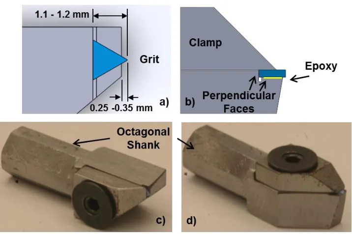
Figure 4-2. Tool Holder: a) Top view and, b) Side view of grit placement with respect to the perpendicular holder surfaces and epoxy placement. c) Grit holder in the negative rake orientation and, d) the Zero rake orientation ... 19

Figure 4-3. Negative rake angle orientation ... 20

Figure 4-4. Microscope Image of Grit Contact Width for Negative Rake Orientation ... 21

Figure 4-5. Zero rake angle orientation ... 21

Figure 4-6. Microscope Image of Two Grit Rake Faces for the Zero Rake Orientation ... 22

Figure 4-7. Halfway Rake Orientation Oblique Rake Faces: Orthogonal to Cutting Direction (left), Top Perspective (right) ... 23

Figure 5-1. Feed Directions ... 25

Figure 5-2. Traverse Feed Experimental Representation ... 26

Figure 5-4. Traverse Experiment at 5 µm Depth and 1 m/s for a Zero Rake Grit on 304 SS

... 29

Figure 5-5. Sample Negative Rake Angle Traverse Experiment at a 12 µm Feed and 1 m/s Speed on 304 SS ... 30

Figure 5-6. Average Cutting and Thrust Forces for Negative Rake Angle Traverse Experiments at a 12 µm Feed and 1 m/s Speed on 304SS ... 31

Figure 5-7. Standard Deviation for Cutting and Thrust Forces at 5µm and 10 µm Depths for Negative Rake Angle Traverse at 12 µm Feed and 1 m/s Speed on 304SS ... 32

Figure 5-8. Maximum Forces for the Negative Rake Traverse Experiments at a 12 µm Feed and 1 m/s Speed on 304SS ... 33

Figure 5-9. 5 µm Depth, Negative Rake Angle: Experimental Data and Base Forces ... 34

Figure 5-10. Negative Rake Traverse Experiment Base Forces at 12 µm Feed and 1 m/s Speed on 304 SS ... 35

Figure 5-11. Plunge Cut Experiment Representation ... 37

Figure 5-12. Grit Contact Area for Plunge Experiment in the Extreme Orientations ... 37

Figure 5-13. Negative Rake Plunge Experimental Forces for Four Experiments at 10 µm Depth of Cut on 304 SS: 1 m/s in a) and b) while 0.1 m/s in c) and d) ... 39

Figure 5-14. Average Forces for Negative Rake Plunge at 10 µm Depth of Cut on 304 SS 40 Figure 5-15. Average Force and Standard Deviation of Negative Rake Plunge at 10 µm Depth of Cut on 304 SS ... 41

Figure 5-16. Maximum Forces for the Negative Rake Plunge Experiments at 10 µm Depth of Cut on 304 SS ... 42

Figure 5-17. 42x Grit Video at 20 µs Shutter Speed: Negative Rake (left), Zero Rake (right) ... 44

Figure 5-18. Grit Variation and Focal Depth at 20 µs Shutter Speed ... 45

Figure 5-19. Chip Formation (left) and Material Build Up (right) ... 46

Figure 5-20. Material Build Up and Resulting Force Increase ... 47

Figure 5-22. Buildup progression of a Negative Rake Plunge at 2.5 µm Depth and 1 m/s

Speed on 304 SS at time: a) 1.524 s, b) 1.575 s, c) 1.625 s, d) 1.637 s ... 50

Figure 5-23. Polished Grit Cutting 304 SS at 1 m/s ... 52

Figure 5-24. Grit at Zero Rake Orientation: Top down view of the rake face (left), Video Image of the side of the grit (right) ... 53

Figure 5-25. Grit Wear Shaping Method: Original (left), after seven passes (right) ... 54

Figure 6-1. Sketch of forces for the Arcona model ... 56

Figure 6-2. Increasing Depth Spiral Experiment with grit profiles every revolution ... 58

Figure 6-3. Polaris CMM and Optical Probe ... 59

Figure 6-4. a) Polaris Cylinder Measurement and b) Unwrapped Polaris Surface ... 60

Figure 6-5. Close upUnwrapped Polaris Measurement for Workpiece Grooves ... 61

Figure 6-6. Polaris Groove Profiles that were Distorted by Interpolation of Poor Data Density and Probe Drop Out ... 62

Figure 6-7. Axial Grit Profile with the Talysurf ... 63

Figure 6-8. Talysurf and Rotary Index Setup for Axial Profile Measurements ... 64

Figure 6-9. Relating forces to workpiece grooves at 0° spindle position (theta) ... 65

Figure 6-10. Grit Profile: a) Top View, b) Side View ... 66

Figure 6-11. Zero Rake Flank Faces a) Top view and the two flank face edges, b) Side view and the flank face ... 68

Figure 6-12. True height measurement for a foreshortened surface [23] ... 68

Figure 6-13. Original and Stretched Flank Face Images ... 69

Figure 6-14. Flank Area Measurement ... 70

Figure 6-15. Negative Rake Flank Area a) Top View and projection of rake area, b) Front view, c) right side view and projection of flank area ... 71

Figure 7-1. Ten Increasing Depth Cutting Experiments at Different Cutting Speeds with Zero Rake Tool on 304 SS (** Experiments were at a Single Depth of Cut) ... 73

Figure 7-2. Zero Rake Speed Comparison for Cutting Forces on 304 SS ... 74

Figure 7-4. 4330 Steel Experimental Cutting Forces with Respect to Chip Area (**

Experiment was at a Single Depth of Cut)... 77

Figure 7-5. 1215 Steel Experimental Cutting Forces with Respect to Chip Area ... 78

Figure 7-6. 52100 Steel Experimental Cutting Forces with Respect to Chip Area ... 78

Figure 7-7. Cutting Force Comparison for Steel Materials at 1 m/s Surface Speed ... 79

Figure 7-8. Thrust Force Comparison for Steel Materials at 1 m/s Surface Speed ... 79

Figure 7-9. Grit Orientation Impact on Cutting Forces ... 82

Figure 7-10. Grit Orientation Impact on Thrust Forces ... 82

Figure 7-11. Zero Rake Orientation Workpiece Profile ... 84

Figure 7-12. Negative Rake Orientation Workpiece Profile ... 85

Figure 7-13. Halfway Rake Orientation Workpiece Profile ... 86

Figure 7-14. Orientation Fracture Forces and Removed Chip Area ... 87

Figure 7-15. Fractures on a 304 SS at 1 m/s for an Increasing Depth Spiral: a) Zero Rake Orientation, b) Halfway Rake Orientation, c) Negative Rake Orientation ... 88

Figure 7-16. Specific Cutting Energy Comparison ... 90

Figure 7-17. Specific Cutting Energy Data Fit for Clarity ... 90

Figure 7-18. Specific Cutting Energy Comparison for 304 SS Speeds ... 91

Figure 7-19. Specific Cutting Energy Comparison for Rake Orientation... 92

Figure 7-20. Specific Cutting Energy Comparison to Depth of Cut for Rake Orientations . 93 Figure 7-21. Chip Speed Calculation Images for a Negative Rake Plunge ... 94

Figure 7-22. Shear Angle Relation to Chip and Workpiece Velocity ... 95

Figure 7-23. Four Contiguous Images for a Zero Rake Increasing Depth Spiral Used to Calculate the Shear Angle ... 96

Figure 8-1. 304 SS Cutting Force: Experiment and Modeled Fit ... 101

Figure 8-2. 304SS Thrust Force: Experiment and Modeled Fit ... 101

Figure 8-3. 4330V Cutting Force: Experiment and Modeled Fit ... 102

Figure 8-4. 4330V Thrust Force: Experiment and Modeled Fit ... 103

Figure 8-5. 1215 Cutting Force: Experiment and Modeled Fit... 104

Figure 8-7. 52100 Cutting Force: Experiment and Modeled Fit... 105

Figure 8-8. 52100 Thrust Force: Experiment and Modeled Fit ... 105

Figure 8-9. Negative Rake Orientation Cutting Force: Experiment and Modeled Fit ... 106

Figure 8-10. Negative Rake Orientation Thrust Force: Experiment and Modeled Fit ... 107

Figure 8-11. AdvantEdge Parameter Description [34] ... 109

Figure 8-12. Tool Geometrical Parameters for a) Zero Rake, b) Negative Rake ... 112

Figure 8-13. Zero Rake Width Approximation for AdvantEdge ... 113

Figure 8-14. 304 SS Speed and Cutting Force Comparisons to Third Wave ... 114

Figure 8-15. 304 SS Speed and Thrust Force Comparisons to Third Wave ... 115

Figure 8-16. Steel Cutting Force Comparisons to Third Wave ... 116

Figure 8-17. Steel Thrust Comparisons to Third Wave ... 116

Figure 8-18. 1215 Cutting and Thrust Comparison to Third Wave ... 117

Figure 8-19. Third Wave Grit Orientation Effect on Cutting Forces at 1 m/s for 304 SS .. 119

Figure 8-20. Third Wave Grit Orientation Effect on Thrust Forces at 1 m/s for 304 SS ... 120

Figure 8-21. Third Wave Grit Orientation on Cutting Forces at 1 m/s for 52100 Steel ... 121

Figure 8-22. Third Wave Grit Orientation on Thrust Forces at 1 m/s for 52100 Steel... 121

Figure 8-23. 304 SS Peak Tool Temperatures at 1, 4, and 8 m/s Cutting Speed ... 123

Figure 8-24. Peak Tool Temperatures of Steel Workpieces ... 124

Figure 8-25. 304 SS Temperature Profile at 1 m/s and 20 µm Depth ... 125

Figure 8-26. 1215 Temperature Profile at 1 m/s and 20 µm Depth ... 125

Figure 8-27. 52100 Temperature Profile at 1 m/s and 20 µm Depth ... 126

Figure 8-28. Negative Rake Orientation for 304 SS at 1 m/s and 20 µm Depth ... 126

Figure 10-1. Camera Focus Locations for: a) Negative Rake Orientation Viewpoint, b) Zero Rake Orientation Viewpoint ... 139

Figure 12-1. Discontinuous Workpieces: 40 mm Contact (left), 3 mm Contact (right) ... 142

Figure 12-2. Load Cell Response (left) and FFT (right) ... 144

Figure 12-3. FFT of Several Load Cell Reponses ... 144

Figure 13-1. Thermocouple Placement on Grit ... 145

Figure 13-3. Analytical Grit Model as a 60° Segment of a Circle ... 147

Figure 13-4. Peak Grit Comparison for Two Measured Temperatures ... 148

Figure 14-1. Grit Holder Dimension Drawing: Units are in Inches ... 149

L

S

Symbol Meaning

µ Friction coefficient between the rake face of the tool and workpiece

µf Friction coefficient at the flank face of the tool and workpiece

µs Specific cutting energy

A Area

Ac Removed chip area

Aexperiment Experimental Area

Af Flank contact area of tool

Aprofile Removed chip area or removed material area

d Depth

E Elastic Modulus

Fc Cutting Force

Ft Thrust Force

G Grinding Ratio

H Hardness of workpiece material

P Power

Pc Cutting Force

Pt Thrust Force

Q Volume removal rate for material

rc Cutting ratio

vchip Chip speed

vcut Workpiece speed or cutting speed

VRemoved Volume of material removed from workpiece

vw Workpiece speed or cutting speed

VWear Volume of wear on abrasive product

Wmodel Width of tool for the model

α Shear angle of the chip

σs Normal Stress

τs Shear Stress

1

B

1.1 MATERIAL REMOVAL PROCESSES

There have been many methods developed to remove excess material from a part or workpiece. These material removal processes have aided innovation by providing the ability to shape parts for complex machines all the way to insignificant household commodities. Understanding and improving specific mechanisms involved with any type of material removal process can give the upper hand to an innovator against competing parties. Small improvements can create better products that remove material more efficiently, which can correlate to larger profit margins.

1.1.1 MACHINING

Machining is characterized by removing material from a workpiece with a harder tool, or a collection of tools, that has a sharp edge. Machining can take many different forms and is categorized by the methods that a workpiece and tool contact and remove material. A few brief examples of different machining methods are given for clarity. Lathing uses a stationary tool with a spinning workpiece to remove material on the outer diameter of the workpiece. A mill uses a rotating tool to remove material as the workpiece moves under it. Grinding uses a collection of sharp abrasive particles to remove material.

geometries. An extensive review of cutting models is given by Shaw [2]. Other models have been developed by Drescher [4] in 1992 and Arcona [5] in 1996 to predict forces in precision machining. However, each model is usually applicable for parameters that are similar to the conditions which the model was based on. Shaw [2] attributes the limits of any model to the over-simplification of the intricate material removal process.

1.1.2 GRINDING

Grinding is a generic term that describes machining with abrasive particles. An abrasive particle is synonymous to abrasive grits or abrasive grains, and shortened further to just a grain or grit. Grinding processes can be further defined by the method that abrasive products are held together. The two main categories of grinding abrasives are bonded and coated abrasives [6,7].

Bonded abrasives include products like grinding wheels and are composed of grits held together by a rigid bonding matrix. Bonded abrasives make up the majority of abrasive products due to their versatility in general grinding, sharpening, and cutting applications. They are used for cutoff applications where material is cut off from ends of workpieces, and in precision applications where the rigid structure of the wheel allows small material removal depths.

Coated abrasives are made up of a single layer of abrasive grits that are attached to a flexible substrate backing material with resin. The substrate material can be a cloth, paper, or polymer material and include products such as an abrasive disk, sandpaper, or abrasive belt. Coated abrasives are used in surface-treatment applications from smoothing and finishing to stock material removal, where a large quantity of material is removed.

1.2 COATED ABRASIVES

promotes more material removal. A first coat of resin is used to hold the grits in place after the electrostatic field is removed and a second coat of resin is used to further secure them [8]. The outer layer of resin completely covers the abrasive grains as shown on the coated abrasive belt in Figure 1-1 (the grits appear as bumps).

Figure 1-1. Coated Abrasive Belt

Figure 1-2. SEM Image of Shaped Alumina Grits [10] (left), Crushed Alumina Grits (right)

1.3 GRINDING PHYSICS

The physics of grinding is similar to machining but has different tool geometry. While milling and lathing tools generally have a single well-defined cutting region that is then worn down by machining, grinding is made of up of many grits acting cooperatively in the cutting process. This is appealing when cutting hard to machine materials. Where a single tool would wear quickly, many cutting tools or abrasive grains wear together and the product as a whole can last longer before it is replaced.

However, there are still challenges with grinding. Individual grits have a different width, depth, length and position [6,11,12] which change the tool/workpiece contact conditions and effect material removal morphologies [13-17]. The geometry variation between grits on a single abrasive product can impact the surface finish quality of a grinding product at identical

machining conditions [9,18].

removal; that is the least energy used per material volume removed. In grinding the majority of the grits either rub or do not contact the workpiece, while only a few grits are actively removing material by cutting [17,20].

Shaw (in Chapter 1) [6] explains that grinding is influenced by the large cutting edge radius of the tool and often times, large negative rake angle. This creates a small region of plastic deformation in the workpiece and chip. The rake angle is shown in Figure 1-3and represents the contact angle of the front face of a tool with respect to a position normal to the workpiece surface. Komanduri [21] also compared grinding of a single grit to cutting with a large negative rake angle tool because of the large cutting edge radius of the grit.

Figure 1-3. Orthogonal Tool Model: Positive Rake (left), Negative Rake (right)

1.4 GRINDING WEAR

Mechanisms of wear in grinding are typically attritious wear, fracturing, and grain pull out [6,8,11,12,22]. Grain pull out was not a mechanism of wear that was studied within this thesis because it occurs at the bonding agent of a grinding belt or wheel, not at an individual grit. Attritious wear is a flattening of the flank face (flank wear) or further dulling of the grit cutting radius. Effects of attritious wear may lead to an increase in forces and lead to grit fracture. Attritious wear can also have a large impact if the cutting tool and workpiece have a chemical affinity. For example, in the case of alumina on steels, flank wear is lower than other materials since the two materials are fairly inert, [8] (in Chapter 22 and 26). Grain fracture can either be small scale, retaining grit shape, or large scale splitting the grit into multiple fragments. The individual microstructure has a large impact on which type of fracture is most common [12] (in Chapter 3).

Wear is typically measured in a product perspective via a grinding ratio, or the volume of material removed from the workpiece, VRemoved, to volume of wear on the abrasive product,

Vwear. A grinding ratio represents the overall performance of a coated abrasive or grinding wheel where the quantitative values of material are significant enough for measurements and comparisons. The grinding ratio is given in Equation (1-1).

(1-1)

1.5 PROBLEM STATEMENT

The research and concepts developed in this thesis sought to provide necessary tools to visualize and evaluate a single abrasive grit during cutting. High speed video was used to capture images of the grit cutting while tool forces were recorded with a load cell. Experimental results were compared to finite element simulations and empirical cutting models to determine the validity of models in a single abrasive application. The goal of this project was to establish methods to distinguish characteristics among tool wear, geometry, temperature and forces based on operating parameters experienced in the grinding process.

2

E

A

2.1 ALUMINUM OXIDE GRIT MATERIAL

The grit material used in the experiments within this thesis is an unknown composition of Aluminum oxide. Aluminum oxide has the general material composition Al2O3 and is also referred to as alumina, corundum and emery. Alumina is a generic term and may refer to a pure alumina substance or may have other material compositions added for improved physical properties. Alumina is known for its physical properties of high hardness and strength. The mechanical properties of alumina are affected by the material microstructure and tend to fail by fracture. The fracture force is dependent on the specific microstructure of the grit; therefore a well-designed grit microstructure could produce fracture at beneficial intervals. For instance, alumina grits are often used for ferrous metals like steel because they have a low chemical affinity to ferrous metals, but also fracture before abrasive wear has much time to negatively affect cutting [6,12].

2.2 ALUMINA GRIT GEOMETRY

Figure 2-1. SEM Image of Alumina Grits on Coated Abrasive [10]

Figure 2-2. Nominal Grit Dimensions on a Carbon Tape Background in a SEM

Figure 2-3. Grit geometry and variability at the scale of cutting

A typical depth of cut may be in the range of 10 µm. Looking at the Figure 2-2 there is variability at the nose with different ridges and high spots on the grit. A case study was done to measure the cutting radius of a specific grit to give the order of magnitude of the grit geometry. The measurement followed the procedure that Lane [23,24] and Shi [25,26] used for measuring diamond tools, called an EBID (Electron Beam Induced Deposition) measurement. The recorded edge radius was 20 µm. This was only used as a general scale relation since individual grits would be different.

2.3 PRECISION LATHE

inch pitch lead screws. The workpiece was attached to the spindle that rotates around the z-axis on an air bearing at speeds ranging from 100 to 1600 RPM.

Figure 2-4. Experimental Setup

Workpieces were thin disks with diameters between 3.5 to 5 inches and thicknesses between 1/32” to 1/4". The workpiece was attached to the DTM spindle. Excess run out of the workpiece was removed before experiments by facing off the workpiece diameter with a carbide tool. A segmented workpiece could replace the cylindrical workpiece for discontinuous cutting experiments. Further orientation and experimental procedure of the grit and workpiece are described in Section 4.

aligned with the center of the workpiece. The grit was held on a tool shank that could be removed from the tool mount for tool wear analysis. The tool mount also held the three-axis load cell used to record cutting forces. A high speed camera with a 36x microscope objective captured the cutting process simultaneously as forces were recorded. A high intensity light source illuminated the grit and chip field of view of the camera for the short exposure times needed for a high frame rate.

2.4 LOAD CELL AND DSPACE SYSTEM

The load cell was a Kistler model 9251A three axis piezoelectric load cell; two axes are in shear and one in compression. The load cell measured cutting, thrust, and side forces that were tangential, normal and axial to the workpiece as shown in Figure 2-5. A diagram of the load cell is given in Figure 2-6.

Figure 2-6. Kistler Model 9251A Piezoelectric Load Cell and Axes [27]

The recorded forces are often referred to together as the cutting forces. The cutting and thrust forces were measured with the shear axes and the side force with the compressive axis. The sensitivity of the compression axis is 4 pC/N and the shear axes were 8 pC/N while the stiffness of the compression axis was 2600 N/µm and the shear axes were 1000 N/µm. The natural frequency of the two shear axes, corresponding to the cutting and thrust forces, was measured to be 11.6 kHz. The load cell was read through a 3 channel, 10 V, Kistler 5004 amplifier. The gain and miscellaneous settings of the amplifier are given in Appendix 12. The load cell and amplifier could measure forces up to 45-50 N.

force signal reached a magnitude of 0.12 V or about 0.5 N. The data that was recorded by the dSpace system was also recorded once the thrust force reached the aforementioned trigger magnitude.

2.5 HIGH SPEED VIDEO SYSTEM AND OPTICS

The high speed camera in Figure 2-4 was aligned with the grit and workpiece to provide high speed imaging of the cutting process. The camera and grit were both positioned on the DTM x-axis so they moved together while the workpiece moved independently on the z axis. The camera was mounted on a stand that could be adjusted for fine focus of the camera. The focus was adjusted by a flexure mechanism shown in Figure 2-7. A screw on the flexure is advanced by 25 µm/rev which causes the flexure to bend and moves the entire camera a few micrometers towards the workpiece. A 36x Newport reflective microscope objective and a 1.2x camera attachment was used to magnify the cutting interface. The combined optical system had a magnification of 43.2x which corresponded to a 440 µm by 330 µm viewing window of the cutting process and depth of view of 30 µm.

The high speed camera is a Phantom Cam v7.3 with a detector array of 800 x 600 pixels that can run at speeds up to 6006 FPS (frames per second). The video camera contained 16 GB (gigabytes) of memory, which corresponds to about 3.4 seconds of continuous video footage at 6006 fps or 6.8 seconds at 3000 fps. The camera was capable of a circular recording buffer, meaning it could record video a set time before and after the trigger time. Information on how the high speed imaging system was used to capture cutting is given in Section 5.4. The shutter speed could be as short as 1 µs. However, as the shutter speed was reduced, more light was required to produce the same image intensity on the detector. The shutter speed was typically set at 10 µs to 20 µs for experiments to provide acceptable images.

The shutter speed had a large impact on motion blur for moving objects in the field of view; a shorter speed could capture faster objects. Clarity of material visualization suffered at long exposure times and resulted in blurred still frame images. The exposure time was balanced to capture both objects in motion and stationary ones. A Prior Lumen 200 light source was directed to the field of view through the top of the microscope mount in Figure 2-7. The light is redirected in the microscope mount to follow the same optical path as the video camera. The light source was a 200 W white light halogen source.

3

P

I

G

M

W

Figure 3-1. First Mounting Techniques and Estimated Wear Pattern

More significant difficulties in early experiments involved problems of grit mounting with epoxy alone. The epoxy was a 3M two part structural epoxy, called DP-460 off white. The DP 460 was cured at 60°C for two hours for maximum bond strength. Two methods of using epoxy to secure the grit are shown in Figure 3-2. Epoxy was placed around and under the grit on a flat mount and also in a small notched hole that fit the tip of the grit. Both methods utilized epoxy as the main source of securing the grit.

Figure 3-2. Epoxy Mounting on a Flat Surface (left) and in a Notched Hole (right)

Figure 3-3. Grit Before Fracture (left), Grit After Fracture (right)

In both methods to secure the grit from Figure 3-2, once cutting and thrust forces were above 20 N either the epoxy was likely to fail or fracture occurred. The forces reached that magnitude because the grit was in contact with the workpiece across about a 0.8 mm width, which created a large chip area. The epoxy failed in tension while the shear stress direction of the epoxy could resist larger forces.

The tensile stress was a direction that lifted the grit from the surface of the holders and the shear stress was in a direction that moved the grit around the mounting surface. For adhesives in general, tensile stress may also be more specifically referred to as peel or cleavage stress for oblique forces with respect to the adhesive layer. Most epoxies have a high shear strength and low tensile strength. The cutting forces employed on the grit were not pure tension or shear but a combination. It was determined that epoxy alone did not have the necessary strength to hold the grit and a different design was needed to constrain the grit.

4

G

G

F

W

E

4.1 GRIT GEOMETRY

extreme grit orientations and one intermediate orientation. The testing orientation also provided an experimental basis for an optimal grit placement. The two extreme grit orientations, shown in Figure 4-1, could create either a zero rake angle or a negative rake angle with respect to the workpiece. Although grit irregularities may not provide a perfect 0° or -30° rake angle, the general rake angle was referenced to distinguish the orientation. Further explanations of the rake angles are described further in Sections 4.3 to 4.5.

Figure 4-1. Extreme Grit Orientations

4.2 TOOL HOLDER DESIGN

Developing a method to support an individual grit (only 1.3 mm along each side) was an important part of the project. A repeatable mounting technique was needed for grit placement for grits that varied slightly in size. For simplicity the grit holder was equipped with two perpendicular faces to ensure the grit was laid flat and flush against the faces as shown in Figure 4-2. The perpendicular faces ensured grit orientation with respect to the large triangular face and edge of the grit. Originally only a clamping system was used when developing the holder design. However, a firm clamp was found to induce extra stress on the

grit that could result in fracture after attachment. Also a clamp alone would not provide sufficient torsional support for a grit with an irregular surface.

Figure 4-2. Tool Holder: a) Top view and, b) Side view of grit placement with respect to the perpendicular holder surfaces and epoxy placement. c) Grit holder in the negative rake

orientation and, d) the Zero rake orientation

The final tool holder used both epoxy and a clamp to hold the grit in place shown in Figure 4-2. The clamp held the grit in compression, resisting possible tensile forces where the epoxy was weak. The epoxy was used to resist twisting and slip in the clamp and would act as shear stress on the epoxy.

extreme orientations, previously shown in Figure 4-1, could be achieved as well as a position in between the extremes at 45°. The grit orientations changed the tool rake angle as discussed in the following sections.

4.3 NEGATIVE RAKE ANGLE ORIENTATION

The negative rake angle orientation had a nominal rake angle of -30° and was oriented with respect to the workpiece shown in Figure 4-3. It is important to note that the rake angle could be larger than -30° due to localized geometry such as an extremely blunt grit. The center of the grit was vertically aligned with the center of the spindle and workpiece.

Figure 4-3. Negative rake angle orientation

Figure 4-4. Microscope Image of Grit Contact Width for Negative Rake Orientation

4.4 ZERO RAKE ANGLE ORIENTATION

The zero rake orientation had the triangular surface of the grit as the rake face. The overall rake angle, excluding any localized geometry differences, created a zero degree rake angle, shown in Figure 4-5. As with the negative rake orientation, a large cutting edge radius would change the localized rake angle. Another factor that could influence the localized rake angle is if the grit had any characteristics resembling a chamfered or curved edge. However, care was taken in experiments to select grits without such characteristics. The grit cutting edge was aligned to the vertical center of the spindle.

The tool width in contact with the workpiece had variability between grits, but it was much more repeatable than the negative rake orientation. The average grit had a triangular tip with about a 60° angle before any wear occurred. The variability of the rake face geometry of two different grits is illustrated in Figure 4-6.

Figure 4-6. Microscope Image of Two Grit Rake Faces for the Zero Rake Orientation

The contact width of the zero rake grits was dependent on the depth of cut. As the depth of cut increased so did the contact width as the triangular edges were moved further into the workpiece. The grits shown in Figure 4-6 were the same grits from Figure 4-4 but in the perspective of the triangular face which is the rake face for the zero rake orientation. The zero rake orientation could be slightly rotated to assist in high speed imaging of the grit. The modified orientation and impact on the video system is described in Section 5.5.2.

4.5 HALFWAY RAKE ANGLE

The arrows represent the material flow along the faces of the grit. The arrow labeled “a” shows the material flow on the rectangular face while the arrow labeled “b” shows the material flow along triangular face. The arrow labeled “a” is on the rake face of the negative rake angle orientation and “b” is on the rake face of the zero rake angle orientation. The left section of Figure 4-7 shows the rake faces from the perspective of the cutting direction while the right gives a top down perspective.

Figure 4-7. Halfway Rake Orientation Oblique Rake Faces: Orthogonal to Cutting Direction (left), Top Perspective (right)

The characteristics of the halfway rake are a combination of the zero and negative rake orientations. An experimental comparison between the rake angles are given in Section 7.3.

5

G

C

A

F

I

5.1 BACKGROUND AND FORCES

forces can be monitored to determine when the workpiece surface finished degrades. The cutting and thrust forces can be related to a model for certain parameters to determine tool edge geometry, as described by Drescher [4] and Arcona [5,28]. This is important with precision machining when the surface finish of a part is a critical parameter. However, after initial experiments it was found that the cutting forces for the alumina grit could not be used to characterize wear with diverse grit geometry.

However, Section 5 was based on the assumption that the grit would cut and wear similarly to orthogonal machining conditions and tools. It was expected that the resulting cutting would produce a steady state force with small variation between experiments due to grit geometry. However results showed that unlike orthogonal machining, there was not a precise steady state force or wear rate. The following sections describe the experiments and results that motivated the development of measurement techniques to compare experimental results described in Section 6.2. The following section describes the process and challenges of using forces to characterize grit cutting.

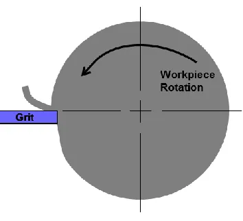
5.1.1 FEED DIRECTION

Figure 5-1. Feed Directions

5.1.2 GENERAL EXPERIMENTAL PROCEDURE

The workpieces were prepared prior to experiments by machining with a carbide tool for a consistent surface finish. The feed rate was related to a theoretical surface roughness of 0.1 µm PV (peak to valley). However, it was discovered that the carbide tool and feed rate produced a PV of 1-3 µm for steel workpieces. The geometry of a new carbide tool had a 400 µm nose radius. The cutting speed for each experiment was determined by the spindle speed and workpiece diameter. The workpiece diameter was measured for each experiment and the spindle speed set to the surface speeds described in the experimental results.

5.2 TRAVERSE EXPERIMENTS AND CHARACTERISTICS

enough to produce overlapping cuts, the contact width of the grit used to remove material was determined by the feed distance per revolution of the workpiece. However, if the geometry of the grit was larger than the feed, it could potentially rub the surface that was just cut. If the grit was an irregular shape, the contact area could be at any point along the grit. Overlapping tool paths were used before groove geometry was measured. In most cases, the traverse feed experiment provided a more consistent and controlled workpiece removal rate in than the plunge experiment.

Figure 5-2. Traverse Feed Experimental Representation

5.2.1 TRAVERSE CUT GRIT EXPERIMENTS

The experiments in Sections 5.2.2 and 5.2.3 were performed with a surface speed of 1 m/s and a traverse cutting feed of 2.38 mm/min. This traverse feed resulted in overlapping tool paths by 12 µm/rev. This only used about 4 % of the 330 µm nominal grit width to remove material for the negative rake orientation. For certain grit geometries, the region of the grit width that was not removing material could rub the workpiece and influence forces. This included grits with flat edges or a large edge radius. Each traverse experiment could potentially reach a cutting distance up to 20 m but could be shortened by fracture or wear.

5.2.2 TRAVERSE CUT CASE STUDY AT THE ZERO RAKE ORIENTATION

The zero rake orientation, described in Section 4.4, was used in a traverse experiment on 304 SS material. Experiments were performed with a surface speed of 1 m/s and a traverse cutting feed of 2.38 mm/min. A traverse feed of that magnitude resulted in overlapping tool paths that corresponded to about 12 µm/rev. There were several cases in which a grit sustained no distinguishable fractures, even after several experimental cutting lengths of 20 m.

Figure 5-3. Zero Rake: Consecutive Traverse Tests at 5µm Depth, 1 m/s Speed, and 12 µm Feed Using a Single Grit on 304 SS

Data points from Figure 5-3 either represent an average force during a single experiment, or several data points representing distinct forces in a single experiment. For instance, experiments that had distinguishable periods of constant force differences, similar to Figure 5-4, were separated into two force averages. Values at 205 m and 211m in Figure 5-3 are representative of the individual experiment in Figure 5-4 where the average forces from 0 to

0 50 100 150 200 250 300 350

-2 -1 0 1 2 3 4 5 6 C u tt in g F o rc e ( N )

0 50 100 150 200 250 300 350

-2 -1 0 1 2 3 4 5 6

Cutting Distance (m)

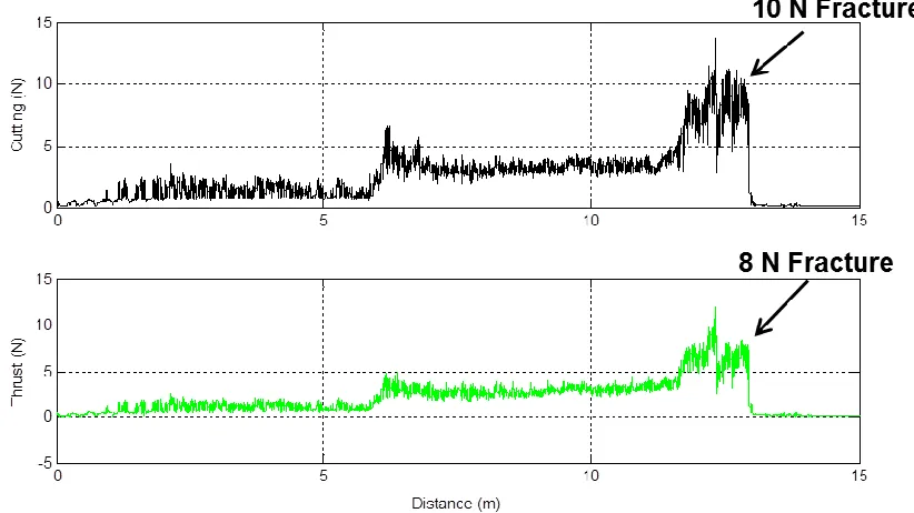
6 m and 6 to 13 m in Figure 5-4 were averaged. Material pickup at the cutting interface was hypothesized to be the cause of the rise in forces at 6 m and 13 m in Figure 5-4. The combination of the forces and high speed video that support this hypothesis is given in Section 5.4.3. The experiment eventually ended in a grit fracture at a 10 N cutting force and 8 N thrust force.

Figure 5-4. Traverse Experiment at 5 µm Depth and 1 m/s for a Zero Rake Grit on 304 SS

Although the forces and standard deviation changed in the experiments, there was nothing to relate the results to, other than assuming the geometry must have arbitrarily changed at fracture. The lack of understanding of cutting geometry involved with the experiments in Figure 5-3 motivated improved experiments described in Section 6.2.

5.2.3 TRAVERSE CUT CASE STUDY AT THE NEGATIVE RAKE ORIENTATION

surface speed of 1 m/s and a traverse cutting feed of 2.38 mm/min. A traverse feed of that magnitude resulted in overlapping tool paths that corresponded to about 12 µm/rev. The experiments consisted of a series of experiments at both 5 µm and 10 µm depths of cut. The negative rake angle orientation proved to expedite fracture events and had significantly shorter periods of continuous cutting compared to the zero rake orientation. A combination of new grits and grits that had recently fractured were used in the experiments. Experiments for the negative rake orientation had highly variable forces as shown in Figure 5-5.

Figure 5-5. Sample Negative Rake Angle Traverse Experiment at a 12 µm Feed and 1 m/s Speed on 304 SS

The irregularity of forces during experiments on the negative rake grit has been partly attributed to material pickup. Visual evidence of material pickup recorded with the high speed video system is described in Section 5.4.3. The data for each trial ended when the grit stopped contacting the workpiece due to a fracture. The overall average force and standard deviation of each test run is given in Figure 5-6 and Figure 5-7 for two grits, one at 5 µm and

5 6 7 8 9 10 11 12

-5 0 5 10 15 20 C u tt in g ( N )

5 6 7 8 9 10 11 12

one at 10 µm depth of cut. The average force was calculated by averaging all the force data of a single experiment pass, effectively taking an average force for all of Figure 5-5. There were no cases of distinct force differences in an individual experiment like was shown in Figure 5-4.

Figure 5-6. Average Cutting and Thrust Forces for Negative Rake Angle Traverse Experiments at a 12 µm Feed and 1 m/s Speed on 304SS

The standard deviation was often larger than the average force due to the large force fluctuations demonstrated in Figure 5-5. The standard deviation data given in Figure 5-7 shows the 5 µm depth experiments, which are the seven experiments shown to the right of the 5 µm mark, and the 10 µm experiments, shown by the five experiments to the right of the

5 10 -2 0 2 4 6 8 10 12 C u tt in g F o rc e ( N )

Depth of Cut (m)

5 10 -2 0 2 4 6 8 10 12

Depth of Cut (m)

10 µm mark. Consecutive experiments were plotted for each grit (at 5 µm or 10 µm depth of cut). As the grit wore and fractured, the variation of experimental forces increased. The variation was attributed to the effect of fracture and material pickup in combination with the grit geometry changing. Even though the two grits were tested with separate depths of cut, 5µm and 10µm, there was no direct correlation between forces and depth of cut. Out of the twelve experiments between the two depths of cut there may have been an average force, but it was indistinguishable with the amount of variation and sample size tested.

Figure 5-7. Standard Deviation for Cutting and Thrust Forces at 5µm and 10 µm Depths for Negative Rake Angle Traverse at 12 µm Feed and 1 m/s Speed on 304SS

For each test run the maximum force, in Figure 5-8, was much larger than the average force in Figure 5-6. Figure 5-8 shows the maximum force from each experiment in the negative

5 10 0 5 10 15 20

Depth of Cut (m)

C u tt in g F o rc e ( N ) 5 10 0 5 10 15 20

Depth of Cut (m)

rake Traverse experiments. The maximum force did not follow any type of trend but often resulted in a grit fracture. Figure 5-8 shows the cutting and thrust forces for thirteen experiments that lead to fracture. The experiments were for 5 µm and 10 µm depth of cut but there is no correlation between the depth and the fracture forces. The variation in the maximum forces could have been due to variable strength grits in conjunction with material pick up. The variance in forces due to material pickup is discussed further in the use of the video imaging system in Section 5.4.3.

Figure 5-8. Maximum Forces for the Negative Rake Traverse Experiments at a 12 µm Feed and 1 m/s Speed on 304SS

To compare experimental force data with consistency further hypothesis were made regarding the effect of material pickup on forces. In several instances the raw force data

5 10

0 20 40 60

Depth of Cut (m)

M a x C u t (N ) 5 10 0 20 40 60

Depth of Cut (m)

showed points in time which the forces appeared to drop to a steady state value. It was hypothesized that the apparent steady state forces were a base force in which there was no material pickup on the tool. If the hypothesis was correct then material pickup on the tool would go through dynamic states of accumulation on the tool followed by a rapid knocking loose of the material. The rapid change to the base force is highlighted in Figure 5-9, originally shown as Figure 5-5. The base force was a short steady state region in the force data that lasted nearly a second in some cases. The base forces were distinguished by the repetitive and seemingly steady force signature.

Figure 5-9. 5 µm Depth, Negative Rake Angle: Experimental Data and Base Forces

Figure 5-10. Negative Rake Traverse Experiment Base Forces at 12 µm Feed and 1 m/s Speed on 304 SS

Experiment forces were not steady state but rather were characterized by rapidly changing forces leading to fracture. Further methods to characterize forces were explored as described in Sections 6 and 7.

5.2.4 TRAVERSE CUT SUMMARY

The overall result of the traverse cutting experiments in both the zero and negative rake orientations was that the experimental data could not be easily related between similar experiments. In fact the actual grit geometry that participated in cutting was unknown. The experimental results revealed the need to define the cutting geometry for each orientation. Defining geometry will improve the basis for which forces can be compared. Later experimental procedures that clarified cutting forces by measuring the grit groove geometry are given in Section 6.

A further outcome of initial experimentation was general grit characteristics were observed which provided initial steps for further testing. A qualitative difference between the orientations was that the negative rake orientation had frequent force spikes which many times resulted in fracture while the zero rake orientation was much more consistent. Another characteristic taken for further experimentation was to use much larger traverse feed rates or non-overlapping traverses. The larger feed rates had a twofold purpose. The first was so tool grooves could be identified but also to increase the overall removed material. The Traverse experiments had a theoretical removed chip area of less than 150 µm2 in all conditions and having a larger removed chip area would provide more distinguishable forces between experiments of different parameters.

5.3 PLUNGE EXPERIMENTS AND CHARACTERISTICS

Figure 5-11. Plunge Cut Experiment Representation

The grit depth of cut was set by advancing the grit a specific distance into the workpiece for each revolution. After the first workpiece revolution the depth of cut was constant as the grit advanced further into the workpiece. In most cases the entire contact width of the grit was used to cut the workpiece in the plunge experiments. However, if the end of the grit was not flat, the contact area would grow over several workpiece revolutions. The grit contact area for the end of a non-uniform grit is shown in Figure 5-12 as the grit advanced further in the radial direction of the workpiece.

After the entire width of the grit contacted the workpiece, the forces should be able to reach a point in equilibrium for the negative rake orientation. However, the zero rake orientation forces would not reach a steady state. As the grit would feed into the workpiece a larger area of the triangular face would contact the workpiece and cause higher forces. The zero rake orientation was not used for plunge experiments for this reason.

An important benefit of the plunge cut was that a small fracture did not result in the end of the experiment since the grit continued to feed into the workpiece. A fracture would stop cutting for a short period of time until the grit fed into the workpiece the distance of the fracture and contacted the workpiece material again. However, a large fracture would stop cutting if the fracture reduced the grit size more than the overall plunge distance or total depth of the experiment.

5.3.1 PLUNGE CUT GRIT EXPERIMENTS FOR THE NEGATIVE RAKE ORIENTATION

The plunge cut experiments were conducted in the negative rake orientation on 304 SS. The negative rake plunge experiments were characterized by large force increases as cutting progressed into the workpiece. Often the experiments lasted only a few seconds before the forces increased rapidly and the grit fractured. In most cases a different grit was used in each experiment, there were a few exceptions when grits sustaining small fractures were reused for another experiment. The plunge cut experiments were set to feed the grit into the workpiece to create a 10 µm cutting depth. The depth may have varied due to uncontrolled material pickup on the grit, which would give a higher apparent depth of cut.

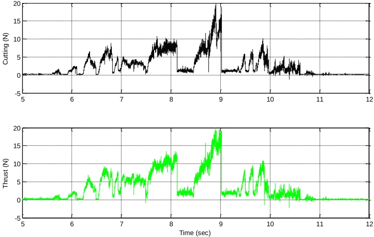
drop in forces without completely stopping cutting. Alternatively a drop in forces could be due to material pickup falling away from the cutting interface. The difficulty of comparing multiple experiments is further shown in the figure. It was determined that the characteristic force rise in separate experiments did not follow a specific pattern. However, there was a qualitative characteristic rise in forces that was linked to material build up at the cutting interface. This was observed with the high speed imaging system described in Section 5.4.

Figure 5-13. Negative Rake Plunge Experimental Forces for Four Experiments at 10 µm Depth of Cut on 304 SS: 1 m/s in a) and b) while 0.1 m/s in c) and d)

average forces as shown in Figure 5-15. The standard deviation plot is separated into the first six experiments at 0.1 m/s, six subsequent experiments at 0.5 m/s and the last two experiments at 1 m/s. Various cutting speeds were used in the plunge cut experiments to reduce motion blur and increase video quality using a shutter speed of 20 µs. When speed was varied there was no distinguishable force trend. The average cutting force for all of the experiments was 2 N and the average thrust force was 2.5 N.

Figure 5-14. Average Forces for Negative Rake Plunge at 10 µm Depth of Cut on 304 SS

0.1 0.5 1

0 2 4 6 8 C u tt in g F o rc e ( N )

0.1 0.5 1

0 2 4 6 8

Cutting Speed (m/s)

Figure 5-15. Average Force and Standard Deviation of Negative Rake Plunge at 10 µm Depth of Cut on 304 SS

The force plots of the plunge experiments from Figure 5-13 were characterized with consecutive fractures where fractures normally occurred at the maximum force. The maximum forces for the experiments are plotted in Figure 5-16. The large force difference illustrates that the nominal cutting parameters could not be used to explain the forces.

0.1 0.5 1

-5 0 5 10 15 Standard Deviation

Cutting Speed (m/s)

C u tt in g F o rc e ( N )

0.1 0.5 1

-5 0 5 10 15

Cutting Speed (m/s)

Figure 5-16. Maximum Forces for the Negative Rake Plunge Experiments at 10 µm Depth of Cut on 304 SS

5.4 HIGH SPEED CAMERA IMAGING

5.4.1 IN PROCESS VIDEO

Recording real time video and force data provided key insights to both grit fracture and cutting, especially events that happened in fractions of seconds. The video footage captured during the grit cutting had great value to it; however the resulting still frame images were of lower quality compared to similar stationary optical microscope images like Figure 4-4 and Figure 4-6. The value of the video was in the rapid accumulation of images at speeds up to 6006 FPS. The video and force measurements were triggered simultaneously when the thrust force signal reached 0.12 V which is equivalent to about 0.5 N. The force and video data were used to correlate effects of material build up, chip formation, and grit fracture. The

0.1 0.5 1

0 10 20 30 40 50

Cutting Speed (m/s)

M a x C u t (N )

0.1 0.5 1

0 10 20 30 40 50

Cutting Speed (m/s)

high speed video camera shutter speed was set to 20 µs for experiments. In a few experiments in Section 7 the shutter speed was set at 10 µs or 15 µs, where video quality permitted.

The traverse cut experiments produced overall poor video quality compared to the plunge cuts. The workpiece in traverse experiments was out of focus in most videos because it moved in the direction corresponding to the camera focal depth. This resulted in a blurred workpiece image and grit/workpiece contact in the majority of recorded videos. Plunge cut experiments were used to improve the video quality of grit cutting. The plunge cut enhanced cutting visualization because both the grit and workpiece were focused on the camera in the negative rake orientation. The front face of the grit was aligned with the front face of the workpiece by focusing the grit surface on the high speed video camera and then moving the workpiece axis until it was also in focus. This provided the best chance for a clear video of the grit/workpiece interaction. However, motion of the chips would sometimes obstruct the viewpoint of the tool and workpiece. Grit geometry also had a pronounced impact on the video image quality as discussed in the following sections.

5.4.2 VIEW OF GRIT AND FOCAL DEPTH

Figure 5-17. 42x Grit Video at 20 µs Shutter Speed: Negative Rake (left), Zero Rake (right)

The negative rake orientation provided a flat, broad face for the focal plane of the video image. Video and images taken during cutting provided a view of events that happened on the front triangular face of the grit. However, the grit width, about 300 µm for the negative rake orientation, was much larger than the focal depth of the optics. This limited the camera focus to the front surface of the grit and only events that were happening near the front surface could be recorded. Inferences on material build up and chip formation along the entire cutting width of the tool contact was not possible.

The 30° angle of the face of the zero rake orientation resulted in a blurred outline of the grit. The zero rake images were focused on a diagonal edge running through the depth of field, and only a blurred outline of the rounded top edge could be seen. With either orientation the camera was focused on the tip of the grit so part of the contact area of the grit was recorded; camera focusing techniques are provided in Appendix 10.2. Even though the entire grit may not be in focus in the zero rake orientation, the cutting interface and chip formation would be recorded with careful focus on the potential contact region.

visualization of the cutting contact region which could not be seen. Although the grit was in focus, the workpiece contact was not, preventing a view of the chip formation. While grits with this type were not ideal candidates for chip video, they may be beneficial for capturing grit fracture if it occurs at the front of the grit. Further optimization of the grit imaging is given in Section 5.5.

Figure 5-18. Grit Variation and Focal Depth at 20 µs Shutter Speed

5.4.3 MATERIAL BUILD UP AND CHIP FORMATION

Figure 5-19. Chip Formation (left) and Material Build Up (right)

Chip formation varied slightly based on grit orientation. In most cases of the negative rake orientation, shown in Figure 5-19, the chip had a defined side edge that was in line with the triangular face of the grit. The chip also has a slight rounded top to it which is out of focus of most videos. The zero rake orientation chips were generally a triangular shape with a vertex pointing away from the grit rake face. The vertex of the chip was in line with the tip of the grit that was removing material. In most videos of the zero rake orientation only the tip of the chip was in focus but it depended on the focusing location. Camera focusing techniques for each orientation is given in Appendix 10.2.

Figure 5-20 shows a negative rake plunge at 0.5 m/s with 10 µm depth of cut when a chip was flowing freely in Figure 5-20a, but the chip formation started to slow down and broaden before leading to it being relatively stationary in Figure 5-20b. Shortly thereafter, the chip built up at the cutting interface and a fracture occurred. The built up chip can be recognized in the still frames by noting that there is a dark empty space above the chip in Figure 5-20a, while Figure 5-20b shows material surrounding the entire cutting interface.

Figure 5-20. Material Build Up and Resulting Force Increase

eventually built up in Figure 5-21b. A chip then began to flow from the apparent location of the built up material in Figure 5-21c and Figure 5-21d. However, the material once again began to build up in Figure 5-21e and Figure 5-21f before a fracture occurred, shown by the large drop in forces.