Initial results of combining GPS occultations with ECMWF global analyses
within a 1DVar framework
E. Robert Kursinski1∗, Sean B. Healy2, and Larry J. Romans1
1MS 238-600 Jet Propulsion Laboratory, California Institute of Technology, Pasadena, CA 91109-8099, U.S.A. 2Numerical Weather Prediction Division (Room 338), The Met Office, London Road, Bracknell RG12 2SZ, U.K.
(Received January 20, 2000; Revised August 28, 2000; Accepted August 28, 2000)
We present results of combining occultation refractivity profiles from GPS/MET with ECMWF global analyses in a 1DVar framework in order to separate the wet and dry contributions to refractivity and assess their impact on the analyzed temperature, surface pressure and specific humidity fields. We find significant zonal mean temperature, surface pressure and humidity differences between the 1DVar solutions and the ECMWF analyses reflecting biases between the GPS refractivities and ECMWF analyses. Large profile-to-profile temperature discrepancies in the tropical lower stratosphere are due to waves not represented in the analyses. The 1DVar solution is generally drier than ECMWF particularly in the southern subtropics. Lack of moisture above 300 hPa in the present model caused the solution to make large adjustments in low latitude surface pressure and tropospheric temperatures to increase upper troposphere densities and compensate for the missing upper level moisture. The discrepancies between the solution and the background and observational data sets represent roughly a 2-sigma level of agreement rather than the 1-sigma level desired in a 1DVar solution. Given the simplicity of our error covariances, our results are promising as a first step. In the future, the error covariances need to be refined and, in particular, to vary with location.
1.
Introduction
We describe a set of initial results of combining GPS oc-cultation refractivity profiles with a set of ECMWF global weather analyses in a 1D variational (1DVar) assimilation scheme. The occultations, which number approximately 800, were acquired by GPS/MET from June 21 to July 4, 1995. One goal here is to derive temperature and moisture profiles from the GPS results using the ECMWF analyses as background information to provide the constraints needed to separate the wet and dry contributions to the refractiv-ity which GPS measures. Alternatively one can view the purpose of this effort as using GPS observations to improve weather analyses. Ultimately this work represents a step to-ward combining the unique features of the GPS observations with other observations and modeling to improve weather forecasting and analyses and our understanding of the be-havior of our climate system.
2.
GPS Occultation Background
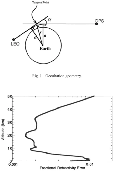
The GPS to low-Earth-orbiter (LEO) occultation geometry is shown in Fig. 1. Relative motion between the transmit-ter and receiver produce a limb scan of the atmosphere in roughly 60 seconds. From measurements of Doppler shift and knowledge of the viewing geometry, the bending angle,
α, and asymptotic miss distance,a, are derived. The index of refraction, n, as a function of radius from the center of
∗Now at Department of Atmospheric Science, University of Arizona,
P.O. Box 210081, Tucson, AZ 85721-0081, U.S.A.
Copy right cThe Society of Geomagnetism and Earth, Planetary and Space Sciences (SGEPSS); The Seismological Society of Japan; The Volcanological Society of Japan; The Geodetic Society of Japan; The Japanese Society for Planetary Sciences.
curvature, r, is derived fromα(a)via an Abelian integral transform relation under the assumption of local spherical symmetry (Fjeldboet al., 1971). At microwave wavelengths refractivity (defined asN =[n−1]106) is given as
where P is pressure, Pw is partial pressure of water vapor,
T is temperature andb1 andb2 are constants equal to 77.6
K hPa−1 and 3.73×10⁵ K2 hPa−1 respectively. Because of its permanent dipole moment, each water vapor molecule contributes approximately 15 to 20 times the refractivity of an average dry (N2or O2) molecule and water therefore
con-tributes significantly to refractivity in the lower troposphere. In the cold, dry conditions of the upper troposphere and above (T < 230 K) water contributes little to refractivity and profiles of refractivity are directly proportional to den-sity. Hydrostatically integrating density yields a profile of pressure (or equivalently geopotential), and knowing density and pressure yields temperature. Given additional tempera-ture information, water vapor can be derived in the middle and lower troposphere.
Coverage and Resolution: A single orbiting GPS re-ceiver with fore and aft antennas can observe between 500 and 700 daily occultations distributed globally, a number which can be roughly doubled by adding a GLONASS re-ceive capability. NASA’s GPS Earth Observatory (GEO) will consist of several orbiting GPS occultation receivers by the end of 2000 including, CHAMP, SAC-C and IOX which will produce more than 1000 occultations per day rivaling the present global radiosonde network but with far more even distribution of coverage. The limb-viewing geometry of the
Fig. 1. Occultation geometry.
Fig. 2. Square root of diagonal terms of the measurement fractional refrac-tivity error covariances.
occultation observations creates a pencil-like sampling vol-ume with along-track resolution of order 200–300 km vertical and cross-track resolution of order 1 km or better as defined by Fresnel diffraction. Sub-Fresnel resolution is achievable through reduction of diffraction effects (Karayel and Hinson, 1997).
Predicted Accuracy: Figure 2 shows the expected frac-tional refractivity errors versus height based on a detailed examination of refractivity, temperature and pressure errors by Kursinskiet al.(1997). Fractional temperature and pres-sure errors are similar yielding sub-Kelvin temperature and
∼10 m geopotential height accuracies from the upper tropo-sphere into the lower stratotropo-sphere. Horizontal gradients are the dominant refractivity error source near the surface and are primarily responsible for the increasing fractional error at lower altitudes. GPS/MET temperatures are consistent with the ECMWF analyses at the 1 to 1.5 K level (Kursinskiet al., 1996; Rockenet al., 1997) while geopotential comparisons with ECMWF are consistent at the 20 m level (Leroy, 1997). Kursinskiet al.(1995) and Kursinski and Hajj (2000a) es-timated the RMS accuracy of water vapor profiles derived from GPS refractivity profiles to be 0.2 g/kg in drier regions increasing to 0.5 g/kg in wetter regions with of the order of 0.1 g/kg depending on the accuracy of assumed temperature.
3.
1DVar Retrieval Overview
Here we briefly summarize the 1D variational approach used in this study. For further details see Healy and Eyre (2000). In a variational retrieval, the most probable at-mospheric state, x, is calculated by combininga priori(or background) atmospheric information,xb, with the measure-ments/observations, yo, in a statistically optimal way. The solution,x, gives the bestfit—in a least squared sense—to both the observations and a prioriinformation. It can be shown in the case of Gaussian error distributions, that ob-taining the most probable state is equivalent to minimizing a cost functionJ(x)given by,
where B is the expected background error covariance
ma-trix; H(x)is the forward model, mapping the atmospheric informationxinto measurement space;EandF are the ex-pected error covariances of measurements and forward model respectively. The superscriptsTand−1 denote matrix trans-pose and inverse. Note that the normalized form has allowed us to combine “apples” (an atmospheric model state vec-tor) and“oranges”(GPS observations of bending angles or refractivity). The error covariance of the solution,x, is
B=[B−1+KT(E+F)−1K]−1 (3)
whereKis∇xyo, the gradient ofyowith respect tox.
Implementation: In this analysis, the measurement vec-tor,yo, is a one dimensional vertical profile of refractivity as a function of geopotential height (yo
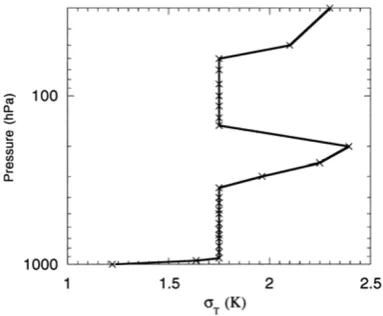
Fig. 3. Square root of diagonal terms of temperature error covariances.
Fig. 4. Square root of diagonal terms of specific humidity error covariances.
The forward model: H(xn): The forward model ‘H’
evaluates a model refractivity value,N, for each‘observed’
geopotential height,zm, using the current state vector esti-mate,xn. The derivation of the refractivity profile from state vector is composed of the following steps. Firstly, the virtual temperature on thefixed pressure levels is calculated. The hydrostatic equation is then integrated, assuming the virtual temperature varies linearly with geopotential height between the pressure levels which enables evaluation of the gradients of log (specific humidity), temperature and virtual tempera-ture with respect to geopotential height. The specific humid-ity, temperature and pressure values can then be calculated at an observation geopotential height,zm. This formulation of the model ensures that the refractivity, pressure, temperature and humidity are continuous over the vertical profile.
Observation Errors: The refractivity measurement error covariance matrix,E, is estimated from Fig. 2. The variance values,σm2, are calculated assuming the percentage error in the refractivity is 1% at the surface and falls linearly with height to 0.2% at 10 km above which the percentage error is constant at this value to 35 km altitude (∼10 hPa). Since the discrete form of the Abel transform is simply a weighted sum of the bending angle values, vertical correlations ex-ist between the refractivity values such that the off-diagonal terms ofE,Enm, are non-zero even if the bending angle
er-rors are uncorrelated. In this work, these are approximated assuming an exponential decay with separation in geopoten-tial height given by, Enm =σnσmexp(−l(zn−zm))where
l is the inverse of a scale length with a numerical value of chosen to be 3×10⁻⁴m−1. This model has been compared with covariances evaluated from the impulse response of an Abel transform routine with the assumption of uncorrelated bending angle errors, and it shows reasonable agreement.
Forward model errors: The forward model in this case is simply the refractivity equation (1) plus the interpolation from the model pressure levels to the observational geopo-tential height levels. The dry part of (1) is accurate to 0.02% and the wet part is accurate to∼1% (Kursinskiet al., 1997). In comparison to other sources of error, these contributions are small and can therefore be ignored. The approach used to interpolate from model pressure levels to observed geopoten-tial heights is very accurate and the interpolation errors will be small to the extent that the model levels are spaced suffi -ciently close to represent the atmospheric structure captured by the observations. Issues regarding model representative-ness (how well can the model actually represent the behavior captured in the observations), and vertical resolution suffi -cient to capture the important aspects of the observations are discussed by Kursinski et al.(2000). For the purposes of the present study, since the errors in the forward model are small, we have set theFmatrix to 0.
4.
1DVar Results Using GPS/MET Data
We have combined refractivity profiles derived from
GPS/MET occultation observations from June 21 to July 4, 1995 with background state vectors from the nearest 6-hour ECMWF analysis, interpolated to the location of each occultation. The data period was chosen because the GPS Anti-Spoofing (AS) encryption was off and the software in the GPS/MET receiver during this period enabled the profiles to extend to within 1 km of the surface much of the time.
We discuss the 1DVar results in terms of temperature, sur-face pressure, and specific humidity differences between the background and solution and in terms of refractivity differ-ences between the observations and solution. The differdiffer-ences are characterized by the mean and standard deviation of their zonal (latitude versus height) behavior.
4.1 1DVar temperature results
Fig. 5. Latitude and height dependence of zonal mean of Background minus Solution temperatures in Kelvin. The black line indicates the zero difference contour.
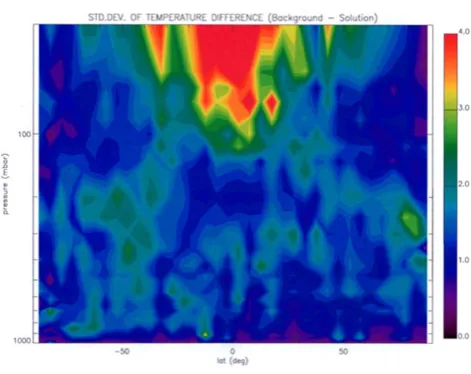
Fig. 6. Latitude and height dependence of zonal standard deviation of Background minus Solution temperatures in Kelvin.
because refractivity should more directly influence specific humidity rather than temperature in warm, wet regions. We believe these changes result indirectly from the lack of water vapor above the 300 hPa level in the model (see Section 5). The low latitude tropopause warming is also a bit surpris-ing and deserves a more thorough examination because we would expect the higher vertical resolution of the GPS re-sults to better capture the extremely cold temperatures at the tropopause than other satellite observations which are assim-ilated into the analyses. Meridional bands also evident in the mean adjustments in tropospheric and stratospheric temper-atures imply the solution is adjusting the temperature lapse rate relative to the background and altering the atmospheric stability.
Near-surface temperatures do not show much change in terms of standard deviation of differences between solution and background temperatures (Fig. 6). Standard deviations in most of the region below the 100 hPa level are in the 1 to
Fig. 7. Latitude dependence of Background minus Solution surface pressure in hPa. Solid line is mean and dashed line is standard deviation.
2.5 K range which is reasonable given that the background temperature errors are roughly 1.7 K (Fig. 3). Standard de-viations in the Southern Hemisphere appear to be somewhat larger than their Northern Hemisphere counterparts in gen-eral. The region of largest standard deviations of more than 4 K in the tropical lower stratosphere reflect the large amount of wave activity in this zone which is apparent in the GPS oc-cultations (Kursinskiet al., 1996; Kursinski, 1997; Tsudaet al., 1999). The 1 to 3 km vertical wavelengths of these waves are resolved by the GPS occultations but not by operational satellite observations or the ECMWF global analyses. The large variations in Figs. 5 and 6 relative to the background er-rors in Fig. 3 indicate that the background temperature error covariances should vary with location.
4.2 1DVar surface pressure results
Figure 7 shows the mean and standard deviation of S−B surface pressure difference versus latitude. North of 50N, the solution has a slightly smaller average surface pressure of about 0.5 hPa than the background generally indicating good agreement where there are relatively many radiosonde observations. South of 45S, the solution surface pressure is larger than that of the background by 1 to 2 hPa. This may reflect a real bias between the analyses and reality but may also reflect the impact of sub-optimal background tem-perature, pressure and specific humidity error covariances at high southern latitudes. Between 40S and 40N, the solution surface pressure is 2 to 4 hPa higher than the background rep-resenting mean shifts in the solution of the order of 1 sigma (=2.5 hPa). The large, mean, low latitude surface pressure adjustments likely result from the lack of model moisture above the 300 hPa level (see Section 5). The standard devia-tion of the surface pressure differences between background and solution are approximately 2 to 3 hPa which is consistent with the 1-sigma (2.5 hPa) background error estimate.
4.3 1DVar specific humidity results
Fig. 8. Latitude and height dependence of zonal mean of Background minus Solution specific humidity in (Background−Solution)/Solution. The black line indicates the zero difference contour.
Fig. 9. Latitude and height dependence of zonal standard deviation of Background minus Solution specific humidity in (Background−Solution)/Solution.
disagreement between model and observations in the indi-vidual profile structure as well as their average. Drying and standard deviations are very large in the southern subtropics between 5S and 30S and 900 and 500 hPa reaching a peak near 15S and 700 hPa consistent with the systematic rounding off of the very sharp PBL top in this area by the background analyses (Kursinski and Hajj, 2000a). Large discrepancies close to 300 hPa near the latitudes of the Inter-Tropical Con-vergence Zone (ITCZ) and Indian-Asian monsoons are likely related to the solution attempting to reconcile the sharp model cutoff in moisture above the 300 hPa level with the observa-tions which have no such cutoff (Section 5). The 10–20% moistening of the solution at high southern latitudes is sur-prising given the low specific humidities there. The 20% moistening near the ITCZ below 500 hPa amid drying in the surrounding regions reflects closer agreement between the model and observed refractivities in this region and probably also reflects some influence from the lack of model moisture
Fig. 10. Latitude and height dependence of zonal mean of Observation mi-nus Solution refractivity normalized to thea prioriobservational refrac-tivity errors defined in Fig. 2. The black line indicates the zero difference contour.
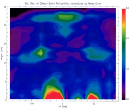
Fig. 11. Latitude and height dependence of zonal standard deviation of Observation minus Solution refractivity normalized to thea priori obser-vational refractivity errors defined in Fig. 2.
above 300 hPa (Section 5).
4.4 Consistency of the measurement and solution re-fractivity structure
may reflect unresolved tropopause structure in the ECMWF analyses. Above 9 km at low latitudes, the solution tends to have less refractivity (lower densities) than observed. In the tropical, lower stratosphere, measurement minus solution standard deviations are larger than 1 sigma likely indicating that the solution was unable to fully represent the waves ob-served in the occultations to within the 1 sigma refractivity errors in Fig. 2. This probably indicates the background tem-perature errors are too small and the vertical resolution in the ECMWF analyses is too coarse in this region.
5.
Impact of No Model Water above 300 hPa
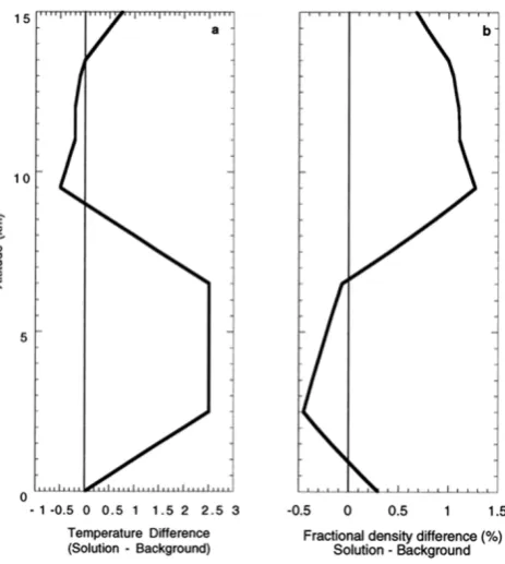
In the 1D model, water vapor extends from the surface to 300 hPa while specific humidities in the real world ex-tend above the 300 hPa level. In the tropical and monsoonal zones, specific humidities at these levels can be 0.5 g/kg or more (Kursinski and Hajj, 2000a), and contribute more than 1% in refractivity. To compensate for the missing water va-por refractivity, the solution must increase the dry density above the 300 hPa level (∼9.5 km altitude) by increasing the pressure at these heights and decreasing the temperature between 300 hPa and 200 hPa (∼12 km altitude). To in-crease hydrostatic pressure at a given altitude, the solution increases temperatures at lower altitudes and increases the surface pressure under the background error covariance con-straints. Figure 12(a) shows a crude representation of the low latitude S−B temperature difference in Fig. 5. With a S−B surface pressure difference of 3 hPa (Fig. 7), the result-ing solution density at 9.5 km is greater than the background by a bit more than 1%, roughly the required compensation amount (Fig. 12(b)).Fig. 12. Simple model of low latitude adjustment in the solution to compensate for lack of water above 300 mb. (a) Temperature dif-ference (Solution−Background). (b) Fractional density difference (Solution−Background).
Features consistent with our hypothesis include 1) the sign change in the temperature bias near 300 hPa in Fig. 5, 2) the coincidence between the meridional extent of large temper-ature modifications in Fig. 5 and high humidities associated with the tropical Hadley circulation, 3) the coincidence of small S−B temperature differences south of 15S and the very dry subsidence zones in the subtropics and 4) the large, negative S−B specific humidity differences near 300 hPa at 5N and 20N in Fig. 8 which are likely due to the overesti-mated dry densities just below 9.5 km altitude as represented in Fig. 12(b). The large hydrostatic modification of densi-ties peaked at 9.5 km in Fig. 12(b) also makes the solution’s results at higher altitudes somewhat suspect.
6.
Impact Summary
The impact of the observations on the solution is reflected in the mean and standard deviations of the solution minus background differences, the contribution to the penalty func-tion and the improved error covariance of the solufunc-tion. Be-cause of the imperfect error covariances and lack of moisture above 300 hPa, some care must be taken in interpretation and drawing conclusions.
The improvement to the error covariance implicit in Eq. (3) reflects background and measurement error covariances and K, the gradient of the observations vector with respect to the model state. Improvement here is estimated as the square root of the variance of the solution divided by the variance of the background for the diagonal terms of the error covariance.
Temperature Improvement: The reduction of the back-ground temperature error in Fig. 13 ranges from very little near the surface to a factor of∼10 near 250 hPa. The largest improvement near 250 hPa whereσTsol/σTbacis 10–15%
re-flects the large error assigned to background temperature es-timates at this altitude associated with the altitude of the tropopause at summer mid-latitudes. The temperature er-ror improvements decrease below the 300 hPa level due to increasing water vapor at lower altitudes. Southern Hemi-sphere temperature improvements are also greater below 300 hPa reflecting the large moisture contrast associated with the winter-summer hemisphere asymmetry.
Surface Pressure Improvement: The new pressure error estimate is 20 to 25% smaller than the background error es-timate with relatively little dependence on latitude except close to the South Pole (Fig. 14). This cannot reflect the whole story because there should be a larger improvement in areas of sparse observations where the background surface pressure uncertainty must larger. Again the background er-ror covariance needs to vary with location to reflect weaker knowledge in poorly observed areas.
Specific humidity Improvement: The specific humidity error in large regions of the troposphere was reduced to less than 60% of the background error (Fig. 15). TheQerror re-duction reaches a maximum in the mid-troposphere near the ITCZ where the solution error is less than 20% of the back-ground error. The biggest disappointment is in the southern subtropics where the relatively small error reduction does not reflect the large mean adjustments in Fig. 8 and substantial discrepancies between the background and solution moisture estimates there in Fig. 9. The reason is the global error co-variance in Fig. 4 does not reflect the systematic ECMWF
Fig. 14. Surface pressure error reduction (σPsolution/σPbackground).
Fig. 15. Specific humidity error reduction (σQsolution/σQbackground).
analysis errors in this region. There are signs that a weaker version of the same problem is occurring near 30N. Regard-ing the general impact on Southern Hemisphere moisture, Kursinski and Hajj (2000b) found the ECMWF analysis spe-cific humidity errors in the Southern Hemisphere to be signif-icantly larger than their Northern Hemisphere counterparts (Fig. 16). Their estimate of the reduction of the background moisture error (Fig. 17) is therefore somewhat larger than that in Fig. 15 in the Southern Hemisphere. Overall the GPS constraints should significantly improve the quality of global moisture analyses.
The magnitude of the penalty function provides some in-dication of the success of the 1DVar. The value of the penalty function achieved here, when normalized by the degrees of freedom (=the number of free parameter in the model), is roughly 4 times larger than optimal implying the solution
re-flects agreement between the background and observations more at the 2-sigma rather than 1-sigma level. Given the simplicity of the error covariances which contain no latitudi-nal dependence and the simple exponential decay refractivity
Fig. 16. Estimated fractional error in ECMWF global specific humidity analyses derived via comparison with GPS results (from Kursinski and Hajj, 2000b).
covariance with diagonal terms taken from Kursinskiet al.
(1997), these initial results described here are encouraging.
Acknowledgments. The authors gratefully thank the GPS/MET program at UCAR for providing the GPS occultation data used in this research. Sean Healy is partially funded by the European Union CLIMAP project (ENV4-CT97-0387). Kursinski and Romans are supported by NASA’s Calibration and Validation (Cal-Val) Pro-gram.
References
Fjeldbo, G. F., V. R. Eshleman, and A. J. Kliore, The neutral atmosphere of Venus as studied with the Mariner V radio occultation experiments, Astron. J.,76, 123–140, 1971.
Gadd, A. J., B. R. Barwell, S. J. Cox, and R. J. Renshaw, Global processing of satellite sounding radiances in a numerical weather prediction system, Q. J. Roy. Met. Soc.,121, 615–630, 1995.
Healy, S. B. and J. R. Eyre, Retrieving temperature, water vapour and sur-face pressure information from refractive index profiles derived by radio occultation: a simulation study,Q. J. Roy. Met. Soc., 2000 (in press). Karayel, E. T. and D. P. Hinson, Sub-Fresnel-scale vertical resolution in
atmospheric profiles from radio occultation,Radio Sci.,32(2), 411–423, 1997.
Kursinski, E. R., The GPS radio occultation concept: theoretical perfor-mance and initial results, Ph.D. thesis, Calif. Inst. of Technol., Pasadena, 1997.
Kursinski, E. R. and G. A. Hajj, A comparison of water vapor derived from GPS occultations and global weather analyses,J. Geophys. Res., 2000a (in press).
Kursinski, E. R. and G. A. Hajj, Zonal variability and accuracy of water vapor estimated from GPS and global weather analyses,J. Geophys. Res., 2000b (submitted).
Kursinski, E. R., G. A. Hajj, K. R. Hardy, L. J. Romans, and J. T. Schofield, Observing tropospheric water vapor by radio occultation using the Global Positioning System,Geophys. Res. Lett.,22, 2365–2368, 1995. Kursinski, E. R., G. A. Hajj, W. I. Bertiger, S. S. Leroy, T. K. Meehan,
L. J. Romans, J. T. Schofield, D. J. McCleese, W. G. Melbourne, C. L. Thornton, T. P. Yunck, J. R. Eyre, and R. N. Nagatani, Initial results of radio occultation observations of Earth’s atmosphere using the Global Positioning System,Science,271, 1107–1110, 1996.
Kursinski, E. R., G. A. Hajj, K. R. Hardy, J. T. Schofield, and R. Linfield, Observing Earth’s atmosphere with radio occultation measurements using GPS,J. Geophys. Res.,102(D19), 23429–23465, 1997.
Kursinski, E. R., G. A. Hajj, S. S. Leroy, and B. Herman, The GPS radio occultation technique, Terrestrial, Atmopsheric and Oceanic Sciences (TAO),11, 53–114, 2000.
Leroy, S. S., Measurement of geopotential heights by GPS radio occultation, J. Geophys. Res.,102, 6971–6986, 1997.
Rocken, C., R. Anthes, M. Exner, D. Hunt, S. Sokolovskiy, R. Ware, M. Gorbunov, W. Schreiner, D. Feng, B. Herman, Y.-H. Kuo, and X. Zou, Analysis and validation of GPS/MET data in the neutral atmosphere,J. Geophys. Res.,102, 29849–29866, 1997.
Tsuda, T., M. Nishida, C. Rocken, and R. H. Ware, A Global Morphology of Gravity Wave Activity in the stratosphere revealed by the GPS occultation data (GPS/MET),J. Geophys. Res., 1999 (submitted).