!
"!" # $ $"
% & ''' (
ISSN No. 0976-5697
Observations on Fault Proneness Prediction Models of Object-Oriented System to
Improve Software Quality
Anil Kumar Malviya
Department of Computer Science & Engineering Kamla Nehru Institute of Technology
Sultanpur, U.P. India [email protected]
Dharmendra Lal Gupta* Research Scholar
Department of Computer Science & Engineering Mewar University, Chittorgarh
(Rajasthan) India [email protected]
Abstract: Software quality is the fundamental need of industry and also for a user. And the future business and reputation of the company depends on the quality of the product. It is need of today to develop quality product. Software quality of system can be measured in terms of fault-proneness of data. Effective prediction for the fault-proneness class early in software development plays a very important role in the analysis of the software quality and balance of software cost.
For the effective prediction of fault-proneness the Pareto Principle will be helpful because it implies that 80% of all errors uncovered during testing will be likely be traceable to 20% of all program components. The problem of course is to isolate these suspected components and thoroughly test them. In this paper, we proposed fault-prone and not-fault-prone class using discriminant analysis , neural network and logistic regression and prediction accuracy was measured and compared for each prediction system.
Keywords: Object-oriented, Reliability, Artificial Neural Networks, Fault, and Failure.
I. INTRODUCTION
Object–oriented technique of software development is becoming de facto standard in software development community. This is due to a variety of claims by many software researchers and practioners that an object oriented approach leads to better productivity, reliability, maintainability and reusability. Object-Oriented systems emphasize three software design fundamentals that are useful in controlling software complexity: polymorphism, encapsulation, and inheritance.
A software complexity model of object-oriented systems was proposed by Tegarden et al. [9]. According to Tegarden software complexity of Object Oriented systems can be described at four levels: variable, method, object, and system. At each level, measures are identified to account for the cohesion (intra) and coupling (inter) aspects of the system at that level.
Software complexity is the difficulty to maintain, change and understand software. It deals with the psychological complexity of programs. Three specific types of psychological complexity that affect a programmer’s ability to comprehend software are problem complexity, system design complexity, and procedural complexity. Design complexity has been conjectured to play a strong role in the quality of the resulting software system in Object Oriented development environments [10]. Prior research on software metrics for Object Oriented systems suggests that structural properties of software components influence the cognitive complexity for the individuals (e.g., developers, testers) involved in their development [11]. This cognitive complexity is likely to affect other aspects of these components, such as fault-proneness and maintainability. Design complexity in traditional development methods involved the modeling of information flow in the application. Hence, graph-theoretic measures [12] and information-content driven measures [13] were used for
representing design complexity. In the Object Oriented environment, certain integral design concepts such as inheritance, coupling, and cohesion have been argued to significantly affect complexity. Hence, Object Oriented design complexity measures proposed in literature have captured these design concepts [6], [14], [15.
Since we all know very well about the Pareto Principle which will be more effective for the prediction of fault-proneness because it implies that 80% of all errors uncovered during testing will be likely be traceable to 20% of all program components. The problem of course is to isolate these suspected components and thoroughly test them.The rest of the paper has been organized as follows. In section 2 we show the related work by different researches. In section 3 we present fault-proneness prediction models. Section 4 discusses software reliability, attributes and faults. In section 5, we discuss confounding effect of class size. Section 6 presents research objectives. Description of the empirical study is presented in Section 7. Results and discussion of the analysis are presented in Section 8. Section 9 concludes the discussion.
II. RELATED WORK
sized Java system, and then apply the model to a different Java system developed by the same team. Fioravanti, F. and Nesi, P. [5] report a research study of more than 200 different object-oriented metrics extracted from the literature with the aim of identifying suitable models for fault proneness class detection. Munson, J.C. [7] describes the processes whereby software complexity metrics may be used to identify regions of software that are fault prone. This information is then exploited to develop a model of dynamic program complexity for the identification of failure prone software. Over the years, increasing importance has been attached to the search of effective models for predicting software faults.
Bingbing, Y. et al. [31] have proposed a new clustering method called affinity propagation is investigated for the analysis of two software metric datasets extracted from real world software projects. The numerical experiment results show that the affinity propagation algorithm can be applied well in software quality prediction in the very early stage and it is more effective on reducing Type-II errors.
Loh, C. H. et al. [32] introduced a software quality model, namely QUAMO (QUAlity Model) which is based on divide-and-conquer strategy to measure the quality of object oriented system through a set of object-oriented design metrics and data mining techniques.
Hribar. L. et al.[34] have proposed about fuzzy logic and KNN (K-nearest-neighbour)[33] classification method approaches are used to predict Weibull distribution parameters shape, slope and total number of faults in the system based on the software components individual contribution.
A wide range of prediction models have been proposed in the literature. Fenton, N. E. et al. [4] provide a critical review of state-of-the-art of models for predicting software defects. Most of the wide range of prediction models uses size and complexity metrics to predict defects. The authors claim that there are a number of serious theoretical and practical problems in many studies. The authors recommended holistic models for software defect prediction, using Bayesian Networks, as alternative approaches to the single-issue models used at present. Cartwright, M. et al. [8] construct useful prediction systems for size and number of defects based upon simple counts as the number of states and events per class. The authors claimed that the prediction system is possible, even in the absence of the suits of metrics that have been advocated by researchers into Object Oriented technology.
To produce high quality object-oriented applications, a strong emphasis on design aspects, especially during the early phases of software development, is necessary. Design metrics play an important role in helping developers understand design aspects of software and, hence, improve software quality and developer productivity [6].
Fault-proneness models can be built using many different methods that mainly belong to few main classes: machine learning principles, probabilistic approaches, statistical techniques, and mixed techniques. Machine learning principles, probabilistic approaches, statistical techniques, and mixed techniques. Machine learning techniques have been investigated by Porter and selby, who studied the use of decision trees [16], [17], and by Khoshgoftaar, Lanning, and Pandya, who applied neural networks [18]. Probabilistic approaches have been exploited
by Fenton and Neil, who propose the use of Bayesian Belief Networks[4]. Statistical techniques have been investigated by Khoshgoftaar, who applied discriminant analysis with Munson [19] and logistic regression with Allen, Halstead, Trio, and Flass[20]. Mixed techniques have been suggested by Briand, Basili, and Thomas, who applied optimized set reduction[21], and by Morasca and Ruhe, who worked by
combining rough set analysis and logistic
regression[22],[23].
III. FAULT-PRONENESS PREDICTION
MODELS
A wide range of prediction models have proposed in the literature. We briefly describe few of the popular methods.
A. Decision Trees
Decision trees are able to identify classes of objects based on a set of local decisions. Each node of a decision tree is associated with an explanatory variable. When a node is reached, the actual value of the associated explanatory variables identifies an output edge that leads to another node. During the classification, the tree is traversed, starting from the root node, until a leaf node is reached. Leaf nodes are associated with classification values. Decision trees can be automatically built from sets of historical observations and are particularly useful when the explanatory variables are discrete, although they can be adapted to handle continuous explanatory variable (in this case intervals are considered) [19].
B. Discriminant Analysis
Discriminant analysis is a statistical modeling technique for estimating classification. It can determine with some accuracy to what extent separation into predefined classes is possible for an observation sample with given metrics, or it can assess the adequacy of a particular classification: it can be predictive or descriptive [24].
The statistical technique of discriminant analysis is basically a classification procedure. The underlying principle of the technique is that an operational hypothesis is formulated that there exists an a priori classification of multivariate observations into two or more groups or sets of observations. Further, the membership in one of these supposed groups is mutually exclusive. A criterion variable will be used for this group assignment. Thus a program, for example, might be classified with a code of zero if it has been found to have no faults or with a code of 1 if it has more than 1 fault [25].
C. Neural Networks
Neural networks are sets of interconnected neurons, each having a number of inputs, an output, and a transformation function. Neural networks are commonly organized in a sequence of layers (at least three), and the neurons of each layer receive as inputs the weighted sum of the outputs of the previous layer. The first layer receives as inputs the explanatory variables and the last layer outputs the resulting classification value. Neural networks natively handle continuous explanatory variables [19].
D. Optimized Set Reduction
the best characterizations of the objects to be assessed. Each of the optimal subsets is then characterized by a set of predicates (a pattern), which can be applied for classifying new objects. Optimized set reduction can handle either continuous or discrete explanatory variables and provides the expected value of the dependent variable [19].
E. Logistic Regression
Logistic regression has been used in empirical software engineering for a number of goals, including estimation of software fault-proneness. Recently, the multivariate logistic regression analysis, whose inputs are several metrics, has been frequently used to evaluate the fault-proneness of the program. A multivariate logistic regression model is based on following relationship equation:
P(X1, …, Xn)=1 / { 1+ exp(-(C0+C1X1+ …+CnXn))}
Where P is the probability that an error is found in a class
and Xis are metrics of the class. If given metrics values make P greater than 0.5, the class is predicted to have faults
(fault prone) [26].
IV. SOFTWARE RELIABILITY, ATTRIBUTES
AND FAULTS
Software reliability is a major component of software quality. The IEEE defines reliability as “The ability of a system or component to perform its required functions under stated conditions for a specified period of time”. According to ANSI, software reliability is defined as the probability of failure free software operation for a specified period of time in a specified environment. A failure is the unacceptable departure of a program operation from program requirements. A software fault is a defect in the code that may cause a failure. It is well known that system reliability is inversely proportional to the number of unfixed defects in the system. Fixing defects may not necessarily make the software more reliable. On the contrary, the process of fault removal may introduce some new faults as it involves modification or writing of new codes. The number of faults remaining in the software at any time is the difference between the number introduced and the number removed. The most effective evaluator of software reliability is a combination of software size and software complexity. It is generally accepted that more complex modules are more difficult to understand and have a higher probability of defects than less complex modules. Given the association between module complexity and errors, it follows that the modules with both a high complexity and large size tend to have the risk because they tend to have code that is very terse making it difficult to either change or modify [7].
There is now sufficient evidence to support the conclusion that there is a distinct relationship between software faults and measurable design attributes and that this information will yield specific guidelines for the design of reliable software. If a software component/module is measured and found to be complex, then it will have a large number of faults. These faults may be detected by analytical methods, e.g. program inspections. The faults may also be identified based on the failures that they induce when the software is executing. Software may preserve a number of latent faults over its lifetime in that the particular manner that it is used may never cause the complex code sequences to execute and thus never expose the faults [7].
The primary objective of modeling the relationship between software design metrics and software faults is that the design metrics may be measured early in the software development life cycle. If we are able to create an appropriate measure of software metrics that is highly correlated with software faults, we may then use this measure of metrics as a surrogate for fault measures in subsequent reliability modeling efforts.
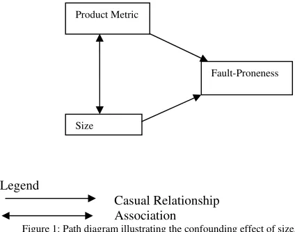
V. CONFOUNDING EFFECT OF CLASS SIZE
A typical empirical validation of object-oriented metrics proceeds by investigating the relationship between each metric and the outcome of interest. In this chapter, we will consider only fault-proneness as an outcome. We define fault-proneness class as the class having at least 1 fault and
Legend
[image:3.612.323.535.250.417.2]Casual Relationship Association
Figure 1: Path diagram illustrating the confounding effect of size.
not-fault-proneness class as the class having no fault. If this relationship isfound to be statistically significant, then the conclusion is drawn that the metric is empirically validated [27]. Resent studies used the bivariate correlation between object-oriented metrics and the number of faults to investigate the validity of the metrics [28]. Also, uni-variate logistic regression models are used as the basis for demonstrating the relationship between object-oriented product metrics and fault-proneness in [29].
However, this approach completely ignores the confounding effect of class size. This can be illustrated with reference to Figure 3. Path (a) is the main hypothesized relationship between the metric and fault-proneness. Here we see that class size (for example, measured in terms of SLOC) is associated with the object-oriented metric (path (c)). Evidence supporting this for many contemporary metrics is found in [29], [30]. Also, class size is known to be associated with the incidence of faults in object-oriented systems, path (b), and is supported in [29], [30]. The pattern of relationships shown in Figure 1 exemplifies a classical confounding effect. This means that the relationship between the object-oriented metric and fault-proneness will be inflated due the effect of size. This also means that without controlling for the effect of size, previous validation studies have been optimistic about the validity of the metrics that they have investigated [27].
Fault-Proneness
VI. RESEARCH OBJECTIVES
In the recent years, Object-oriented approach to software development is becoming very popular in today’s software development environment. The importance of deletion and removal of defects prior to customer delivery has received increased attention due to its potential role in influencing customer satisfaction and the overall negative economic implications of shipping defective software products [6]. In the realm of object-oriented systems, one approach to identify faulty classes early in development is to construct prediction models using object-oriented metrics. Such models are developed using historical data, and can be applied for identifying potentially faulty-classes in future applications or future releases. The usage of design metrics allows the organization to take mitigating actions early such as a redesign and consequently avoid costly rework [2]. To achieve the objectives, the present study aims to elucidate; (i) the relationship between object-oriented metrics and the number of faults present in the class, (ii) the confounding effect of class size on the relationship between metrics and fault prediction, (iii) to derive fault prediction model and (iv) to identify fault-prone and not-fault-prone classes in the object oriented system.
VII. DESCRIPTION OF THE EMPIRICAL STUDY
A. Description of the System Study
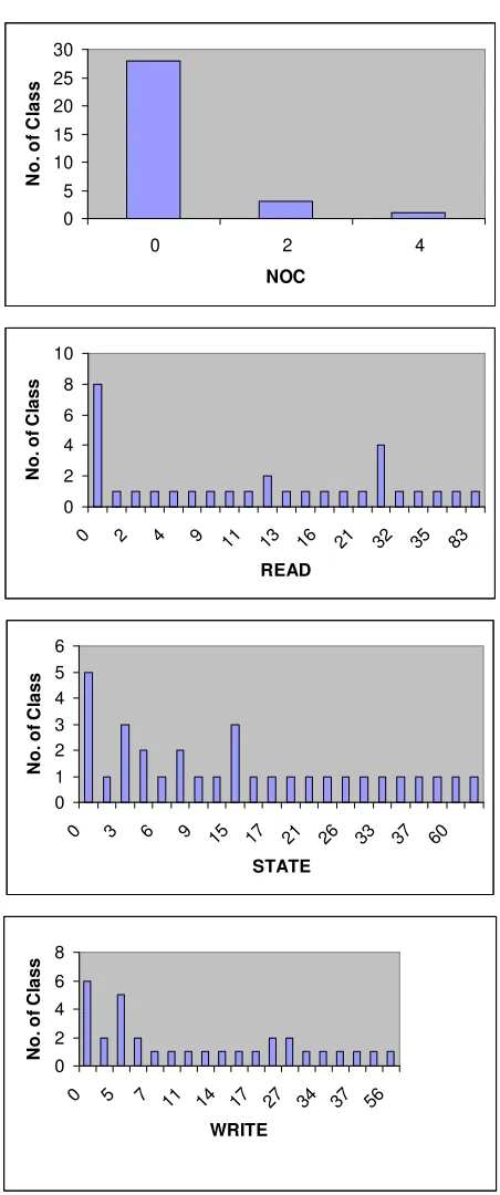
One of the goals of this study is to analyze empirically the object oriented metrics for the purpose of evaluating whether or not these metrics are useful for predicting the probability of detecting faulty classes. The system and raw data used in this study has been taken from [8]. The system studied is a subsystem of a much larger industrial real-time telecommunications system which is comprised of several million lines of code (LOC) and has been evolving over the past 10 years. Its success is central to the Organization’s financial health. The subsystem is written in C++ and has been designed using the Shlaer-Mellor method. It consists of 32 classes which correspond to slightly over 133,000 LOC [8]. Figure 2 shows the distributions of the analyzed metrics based on 32 classes present in the studied system. Figure 3 shows the distribution of defect over the 32 classes of the studied system.
B. Dependent and Independent Variables
The dependent variable (Metric) is the number of faults (DEFECT) in a class. The independent variables (Metrics) used in this study are ATTRIB, STATE, EVNT, WRITES, DELS, RWD, DIT, NOC, LOC, LOC_B, and LOC_H. These dependent and independent variables are described below.
[a] Attributes (ATTRIB): It is defined as the count of attributes per class from the information model.
[b] States (STATE): State variable is defined as the count of states per class in the state model.
[c] Events (EVNT): Events variable is defined as the count of events per class in the state model.
[d] Writes (WRITES): It is defined as the count of all write accesses by a class contained in the CASE tool. [e] Deletes (DELS): It is defined as the count of all delete
accesses by a class contained in the case tool.
[f] Read/write/deletes (RWD): It is defined as the count of synchronous accesses (i.e. the sum of READS, WRITES and DELS) per class from the CASE tool. [g] Depth of Inheritance Tree (DIT) : It is defined as the
depth of a class in the inheritance tree where the root class is zero.
[h] Number of Children (NOC) : It is defined as the number of child classes.
[i] Lines of code (LOC) : It is defined as the number of lines of code per class.
[j] Lines of code (body)(LOC_B): It is defined as the body file lines of code per class.
[k] Lines of code (header)(LOC_H): It is defined as the header file lines of code per class.
[l] Defects (DEFECT) : It is defined as the count of defect per class.
C. Data Analysis Procedure
The procedure used to analyse the data for achieving the aim of the chapter is described in 4 stages.
[a] Descriptive Statistics
The distribution and variance of each measure is examined to select those with enough variance for further analysis.
[b] Correlation Analysis
A correlation coefficient measures the strength of a linear association between two variables.
[c] Univariate Analysis
Univariate regression analysis looks at the relationship between each of the independent variables and dependent variable under study. This is a first step to identify types of independent variables that are significantly related to dependent variable and thus are potential predictors to be used in the next step.
[d] Multivariate Analysis
Multivariate analysis also looks at the relationships between independent variables and dependent variable, but considers the former in combination, as covariate in a multivariate model, in order to better explain the variance of the dependent variable and ultimately obtain accurate prediction.
In this study, we use univariate and multivariate regression analysis for making fault prediction model for estimating no. of fault at a class level of object oriented system using structural design measures. In this paper fault proneness is defined as the probability of detecting a fault in a class. We choose three classification technique discriminant analysis (described in section 3.2), neural networks (described in section 3.3) and logistic regression (described in section 3.5) for classifying the fault-prone and not-fault prone classes of object-oriented system and we also compared the predictability of these methods. We introduce the following three criterion (goodness of fit) to evaluate the result of the prediction [26], [27].
[e] Best Overall Completeness
Overall completeness is defined as the proportion of modules (classes) that are classified correctly:
predicted non-faulty modules and M is the total number of modules. This parameter measures the ability of modules to correctly classify the target software modules (classes), regardless of the category in which the models have been classified.
[f] Best Faulty Module (Class) Completeness
Faulty module completeness is defined as the proportion of faulty modules that are correctly classified as faulty by the model.
faulty module completeness=CPFM/FM
where, CPFM is the number of correctly predicted faulty modules and FM is the total number of actual faulty modules. This parameter measures the ability of the models to identify the most fault-prone part (class) of the target software.
[g] Best Faulty Module (Class) Correctness
Faulty module (class) correctness is defined as the proportion of faulty modules (classes) within the set of modules that are classified as faulty by the model.
faulty module correctness=CPFM/PFM
where, CPFM is the number of correctly predicted faulty modules (classes) and PFM is the total number of predicted faulty modules (classes). This parameter measures the efficiency of a model, in terms of the percentage of actually faulty modules (classes) among the ones that are candidates for further verification.
VIII. RESULTS AND DISCUSSION
A. The first step of the analysis was to produce descriptive statistics (Table-1) of all the variables (independent and dependent). The Table1 shows mean, median, Std. dev., IQR (inter-quartile range), and the number of observations that are not equal to zero. It is noticeable that, since the median value is, in all cases, lower than the mean, each variable exhibits some tendency to skew positively. This is the consequence of a few very large classes. Skewness value ranges from .997 to 3.049 with Std. Error .414.
B. The second analysis step was to calculate spearman rank correlation coefficient of object oriented metrics and number of defect of a class. Results (Table-2) revealed that ATTRIB, and NOC are not significantly correlated to number of defect of a class. Therefore, they were excluded from further analysis. But DEL, DIT, EVNT, READ, WRITE, RWD, LOC, LOC_B and LOC_C emerged to be significantly positively correlated (each at = .01 level) to number of defect of a class.
C. The third analysis step was to look the confounding effects of size. Table-3 depicts confounding effects of size (LOC) on the metrics. All seven selected variables are significantly correlated with number of defect of a class. Therefore, the relationship between the first and the second variable by the theory include the variation due to third variable; hence the probable influences (effect) of the third variable was partially out to estimate the true relationship between the first and the second variables. Analyses (Table-3) disclosed the fact that seven predictors (DEL, DIT, EVNT, READ, STATE, WRITE and RWD) without size control made their significant contributions, and when controlling for
size was estimated, DEL, DIT, EVNT, WRITE, and RWD at level .01 and READ at .05 level demonstrated their significant contributions except STATE metrics. D. The next analysis step was to investigate the
relationship of design metrics and number of fault in a class. Table-4 shows the R2, Adjusted R square, F-ratio and Std. Error of estimate of the system described in section 6. Here, we show individual relationship of design metrics (DEL, DIT, EVNT, READ, STATE, WRITE AND RWD), and size metrics (LOC, LOC_B, LOC_H) to number of fault in a class. Results (Table-4) demonstrated that each predictor individually emerged to show their significant contribution (p<.001 level) to number of defect (fault) in a class, and that all the predictors together, emerged to explain a total of 94% of variance. Here one crucial observation deserves mention that EVNT explained a total of 87% of maximum variance among all of the independents variables under observations. At the end of implementation, the LOC, LOC_B and LOC_H distributively explained 62%, 62% and 58% of variance. Still further, at the implementation level of the system, when all the metrics and LOC metric (leaving LOC_B and LOC_H because of orthoganality) were taken together, a total of 94% could be explained. These observations would provide a tentative idea about number of defect may be encountered in the class of object-oriented system at the time of testing the system. E. Keeping in view the observations, and the one of the
objectives of the study, the early fault prediction model was attempted. The regression equation to predict the number of fault in a class using regression coefficients was found as given below:
defect=-2.24+.19 DEL + 4.47 DIT + .358 EVNT - .06 STATE + .116 WRITE - .126 READ ---(1)
defect=-.58+.42 EVNT ---(2)
The regression model (equation(1)) suggests that Metrics DEL, DIT, EVNT, STATE, WRITE and READ are known, the number of defect(fault) in a class could be estimated at 94% of total variance. The regression equation (2) suggests that if EVNT is known, the number of defect of a class could be estimated at 88% of total variance.
F. Table 5 shows the obtained fault-prone class prediction model by the discriminant analysis. For example, in Table 5, 13 classes are predicted to be not-faulty and actually faulty. Two classes are predicted to be not-faulty but actually not-faulty. The overall completeness and faulty module (class) completeness are respectively 93.8 % and 89.5%. The Table 6 shows the cross-validation results. The cross-cross-validation is done only for those cases in the analysis. In cross validation, each case is classified by the functions derived from all cases other than that case. Results (Table-6) demonstrated that 12 classes out of 13 are predicted to be not-faulty and actually not-faulty. Four classes are predicted to be not-faulty but actually faulty. The overall completeness and faulty module (class) completeness are respectively 78.9% and 84.4%.
be not-faulty but actually faulty. The overall completeness and faulty module (class) completeness are respectively 96.68% and 94.74% greater than the fault-prone class prediction model using discriminant analysis.
H. Table 8 shows the obtained fault-prone class prediction model by the Neural Network. For example, in Table 8, 12 classes are predicted to be not-faulty and actually not-faulty. One class is predicted to be not-faulty but actually faulty. The overall completeness and faulty module (class) completeness are respectively 93.75 % and 94.74.
IX. SUMMARY AND CONCLUSIONS
Cartwright and shepperd (2000) data was reanalyzed to find early indices of predictability of fault-prone classes and number of faults in modules (classes) of object-oriented system. The results may summarily concluded as follows: (i) the DEL, DIT, EVNT, READ, WRITE, STATE and RWD metrics emerged to be significantly correlated to the number of defect (fault) in the class, (ii) each predictor individually emerged to show their significant contribution to the number of fault(defect) in a class, and all predictors together emerged to explain a total of 94% of variance. EVNT metrics individually explained 87% of variance among all of the independents variables under observations. The size metrics (LOC) explained 62% of variance, (iii) the individual predictor DEL, DIT, EVNT, READ, STATE and WRITE without size control made their significant contributions, and when controlling for size (LOC) was estimated DEL, DIT, EVNT and WRITE at p-level .01 and READ at .05 level demonstrated their significant contributions except STATE metrics, (iv) the early fault-prone class prediction model was derived using discriminant analysis, multivariate logistic regression technique and Neural Network with overall completeness and faulty class completeness 93.8% , 96.88 and 93.75 and 89.5%, 94.74% and 94.74% respectively.
[image:6.612.307.559.52.770.2]Our results indicate that DIT (CK-suite metric) and other metrics DEL, EVNT, READ, STATE and WRITE available by the design stage were strongly associated with fault-proneness. Furthermore, the prediction model that we constructed with these metrics has good accuracy. Further extended studies are desirable in support of the findings.
Table 1 :Descriptive Statistics
Mean Median Std. Dev. IQR NOBS<>0
Attrib 8.656 4.500 8.8340 10.750 32
DELS 1.500 1.000 1.3912 2.000 24
DIT 0.438 0.000 0.7156 1.000 10
EVNT 20.531 10.500 26.2948 30.500 27
NOC 0.313 0.000 0.8958 0.000 4
READ 16.250 11.500 19.9192 26.250 24
STATE 18.031 13.000 22.9368 22.250 27
WRITE 14.219 8.500 14.4507 20.500 26
RWD 31.969 22.000 33.6917 47.000 27
LOC 4178.500 3254.500 3981.3226 4055.750 32
LOC_B 3427.594 2775.5 3427.1528 3502.50 32
LOC_H 750.906 707.00 556.9252 552.26 32
Table 2 : Spearman Rank Correlation
ATT RIB
DEL S
DIT EVN T
NO C
READS STATE S
WRI TES ATTRIB 1.00
DELS -0.12 1.00
DIT -0.34 0.46 1.00
EVNT 0.32 0.53 0.38 1.00
NOC 0.26 -0.41 0.09 0.34 1.00
READS 0.49 0.50 0.36 0.88 0.18 1.00
STATES 0.56 0.50 0.10 0.90 0.25 0.87 1.00
WRITES 0.53 0.57 0.38 0.81 0.09 0.94 0.82 1.00
DEFECT 0.17 0.62 0.58 0.84 0.18 0.76 0.75 0.77
LOC 0.56 0.48 0.14 0.91 0.31 0.86 0.97 0.80
LOC_B 0.56 0.48 0.14 0.91 0.31 0.87 0.97 0.80
LOC_H 0.62 0.48 0.10 0.88 0.26 0.87 0.98 0.80
DEFECT LOC LOC_B LOC_H
DEFECT 1.00
LOC 0.76 1.00
LOC_B 0.76 1.00 1.00 LOC_H 0.76 0.99 1.00
Table-3 : Confounding Effect of Class Size
S. No. Metrics Without Size Control Controlling for size (LOC)
Correlation p-value Correlation p-value
1. DEL .619 .000 .5732 .001
2. DIT .580 .000 .8545 .000
3. EVNT .838 .000 .8691 .000
4. READ .764 .000 .4083 .023
5. STATE .751 .000 -.1069 .567
6. WRITE .770 .000 .6674 .000
7. RWD .769 .000 .6219 .000
Table-4 : Regression Models:
Model Metrics Rsquare Adjusted Rsquare
Fvalue P-value Std. Error of Estimate M1 DEL .246 .220 9.767 .004 10.472
M2 DIT .307 .283 13.265 .001 10.039
M3 EVNT .876 .872 212.612 .000 4.240
[image:6.612.56.296.547.735.2]M5 STATE .583 .569 41.905 .000 7.788
M6 WRITE .753 .745 91.598 .000 5.988
M7 RWD .761 .753 95.304 .000 5.900
M8 LOC .622 .609 49.328 .000 7.414
M9 M1-M6 .948 .935 75.789 .000 3.01
M10 M9+M8 .948 .933 62.972 .000 3.06
Table-5 : Faulty (class) Prediction in Confusion matrix (Using discriminant analysis)
Prediction Not-faulty Faulty Predictio
n %
Actual
Not-Fault
13 0 13 100 %
Faulty 2 17 19 89.5 %
15 17 32
Overall 93.8 %
Model with all metrics, cut off to .05. The reported numbers are related to faulty classes and not to the number of faults identified.
Table-6 : Fault (class) Prediction in Confusion matrix (Using discriminant analysis)
Prediction Not-faulty
Fault y
Predictio n %
Cross-validated
Not-Fault 12 1 13 92.31 %
Faulty 4 15 19 78.9 %
16 16 32
Overall 84.4 %
Model with all metrics, cut off to .05. The reported numbers are related to faulty classes and not to the number of faults identified.
Table-7 : Fault (class) Prediction in Confusion matrix (Using logistic regression)
Prediction
Not-faulty
Faulty Predictio
n %
Actual Not-Fault 13 0 13 100 %
Faulty 1 18 19 94.74 %
14 18 32
Overall 96.88 %
Model with all metrics, cut off to .05. The reported numbers are related to faulty classes and not to the number of faults identified.
Table-8 : Fault (class) Prediction in Confusion matrix (Using Neural Network)
Prediction
Not-faulty
Faulty Prediction
%
Actual Not-Fault 12 1 13 92.31 %
Faulty 1 18 19 94.74 %
13 19 32
Overall 93.75 %
Model with all metrics, cut off to .05. The reported numbers are related to faulty classes and not to the number of faults identified.
0 2 4 6 8 10
1 3 5 7 11 14 17 24 32
ATTRIB
N
o
.
o
f
C
la
s
s
0 2 4 6 8 10 12 14
0 1 2 3 5
DEL
N
o
.
o
f
C
la
s
s
0 5 10 15 20 25
0 DIT1 2
N
o
.
o
f
C
la
s
s
0 1 2 3 4 5 6
0 2 5 10 12 23 31 39 53 71
EVNT
N
o
.
o
f
C
la
s
0 5 10 15 20 25 30
0 2 4
NOC
N
o
.
o
f
C
la
s
s
0 2 4 6 8 10
0 2 4 9 11 13 16 21 32 35 83
READ
N
o
.
o
f
C
la
s
s
0 1 2 3 4 5 6
0 3 6 9 15 17 21 26 33 37 60
STATE
N
o
.
o
f
C
la
s
s
0 2 4 6 8
0 5 7 11 14 17 27 34 37 56
WRITE
N
o
.
o
f
C
la
s
s
Figure 2: Distribution of the analyzed software metrics. The X-axes represents the value of the metric. The Y-axes represents the number of class.
0 2 4 6 8 10 12 14
0 2 6 10 25 27 47
DEFECT
N
o
.
o
f
C
la
s
[image:8.612.61.287.43.583.2]s
Figure 3: Distribution of the defect metric. The X-axis represents the value of the defect metric. The Y axis represents the number of class.
X. REFERENCES
[1] Briand, L.C., Wust, J., Daly, J.W. and Porter, D.V., “Expolring the Relationships between Design Measures and Software Quality in Object-Oriented Systems”, The Journal of Systems and Software, Vol. 51, 2000, pp. 245-273.
[2] Briand, L.C., Melo, W.L. and Wust, J., “Assessing the Applicability of Fault-Proneness Models Across Object-Oriented Software Projects”, ISERN Report No. ISERN-00-06, Version 2.
[3] EI-Emam, K. El and Melo, W.,“The Prediction of Faulty Classes Using Object-Oriented Design Metrics ”, National Research Counsil Canada, Nov. 1999. [4] Fenton, N.E. and Neil, M., “A Critique of Software
Defect Prediction Models”, IEEE Transactions on Software Engineering, Vol. 25, No. 5, September / October 1999, pp. 675-688.
[5] Fioravanti, F. and Nesi, P., “A Study on Fault-proneness detection of Object-Oriented Systems”, Department of Systems and Informatics, University of Florence, Internet.
[6] Subramanyam, R. and Krishnan, M.S., “Empirical Analysis of CK Metrics for Object-Oriented Design Complexity: Implications for Software Defects”, IEEE Transactions on Software Engineering, Vol. 29, No. 4, April 2003, pp. 297-310.
[7] Munson, J. C., “Software faults, software failures, and software reliability modeling”, Information and Software technology Vol. 38, 1996, pp.687-699. [8] Cartwright, M. and Shepperd, M., “An Empirical
Investigation of an Object-Oriented Software System”, IEEE Transactions on Software Engineering, Vol. 26, No. 8, August 2000, pp. 786-796.
[9] Tegarden, D.P., Sheetz, S.D., Monarchi, D.E., “A Software complexity model of object-oriented systems”, Decision Support Systems, Vol. 13, 1995, pp. 241-262.
[10] Booch, G., “Object-Oriented Analysis and Design”, Second Edition, Benjamin Cummings.
[11] Briand, L. C., Wuest, J., Ikonomovski, S. and Lounis, H.,“Investigation of Quality Factors in Object-Oriented Designs: An Industrial Case Study,” Proc. Int’l Conf. Software Engineering, 1999, pp. 345-354. [12] McCabe, T.J., “A Complexity Measure”, IEEE
Transactions on Software Engineering, Vol. SE-2, Dec. 1976, pp. 308-320.
[image:8.612.323.553.55.173.2][14] S.R. Chidamber and C.F. Kemerer, “Towards a Metric Suite for Object Oriented Design,” Proc. conf. Object Oriented Programming Systems, Languages, and Applications (OOPSLA ’91) Vol. 26, no. 11, 1991, pp. 197-211.
[15] Chidamber, S.R. and Kemerer, C.F., “A metrics Suite for Object Oriented Design”, IEEE Transactions on Software Engineering, Vol. 20, No.6, June 1994, pp. 476-493.
[16] Selby, R.W. and Porter, “Learning from examples: Generation and Evaluation of Descision Trees for Software Resources Analysis”, IEEE Transactions on Software Engineering, Vol. 14, No. 12, Dec. 1988, 1743-1757.
[17] Witten, I.H. and Frank, E., “Data Mining: Practical Machine Learning Tools and Techniques with Java Implementa tions”, Morgan Kaufman Publishers, 2000. [18] Khoshgoftar, T.M., Lanning, D.H. and Pandya, A.S.,
“A Comparative-Study of Patter-Recognition Techniques for Quality Evaluation of Tele communications Software”, IEEE Journal on Selected Areas In Communications, Vol. 12, No. 2, 1994, pp. 279-291.
[19] Denaro, G. and Pezze, M., “Towards Industrial Relevant Fault-Proneness Models”, International Journal of Software Engineering and Knowledge Engineering, Vol. 0, No. 0 (1994) 000-000, © World Scientific Publishing Company.
[20] Khoshgoftar, T.M., Allen, E.B., Halstead, R., Trio, G.P. and Flass, R. M., “Using Process History to Predict Software Quality”, Computer, Vol. 31, No.4, Apr. 1998, pp.66-72.
[21] Briand, L., Basili, V., and Thomas, W., “A Pattern Recognition Approach for Software Engineering Data analysis”, IEEE Transactions on Software Engineering, Vol. 18, No.11, 1992, pp.931-942.
[22] Denaro, G. and Pezze, M., “An Empirical Evaluation of Fault-Proneness Models”, Internet.
[23] Morasca, S. and Ruhe, G., “A Hybrid Approach to Analyze Empirical Software Engineering Data and its Application to Predict Module Fault-proneness in Maintenance”, The Journal of System and software, Vol. 53, No.3, Sep. 2000, pp.225-237.
[24] Hochman, R. and Hudepohl, J. P., “Evolutionary Neural Networks: A Robust Approach to Software Reliability Problems”, Internet.
[25] Munson, J. C. and Khoshgoftaar, T.M., “The Detection of Fault-Prone Programs”, IEEE transactions on Software Engineering, Vol. 18, No.5, May 1992, pp. 423-433.
[26] Kamiya, T., Kusumoto, S. and Inoue, K., “Prediction of Fault-Proneness at Early Phase in Object-Oriented Development”, Internet.
[27] Benlarbi, S., Eman, K.E., Goel, N., “Issues in Validating Object-Oriented Metrics for Early Risk Prediction”, ISSRE Copyright, 1999 Internet.
[28] Binkley, A. and Schach, S., “Validation of the Coupling Dependency Metric as a Predictor of Run-Time Fauilures and Maintenance Measures”, In Proceedings of the 20th International Conference on Software Engineering”, 1998, pp. 452-455.
[29] Briand, L. Wuest, J., Ikonomovski. S. and Lounis, H., “A Comprehensive Investigation of Quality Factors in Object Oriented Designs: An Industrial Case Study”, International Software Engineering Research Network technical report ISERN-98-29, 1998.
[30] Schlesselman, J., “Case-Control Studies: Design, Conduct, Analysis”, Oxford University Prss, 1982. [31] Yang. Bingbing, Yin. Qian, Xu Shengyong, and Guo
Ping, “2008 International Joint Confrence on Neural Networks (IJCNN 2008)”.
[32] Loh. Chuan Ho, Lee Sai Peck, “2009 International Conference on Information Management and Engineering”.
[33] Leif E. Peterson, “K-nearest neighbor”, Scholarpedia, 4(2):1883.(2009),
http://www.scholarpedia.org/article/k-nearest_neighbor. [34] Haribar Lovre, Duka Denis,“Software Component Quality Prediction using KNN and Fuzzy Logic”, International Conference MIPRO 2010,May 24-28,Opatija,Croatia.
About Authors:
Dr. Anil Kumar Malviya is an Associate Professor in Computer Science & Engineering Department at Kamla Nehru Institute of Technology, (KNIT), Sultanpur. He received his B.Sc. & M.Sc. both in Computer Science from Banaras Hindu University, Varanasi respectively in 1991 and 1993 and Ph.D. degree in Computer Science from Dr. B.R. Ambedkar University, Agra in 2006. He is Life Member of CSI, India. He has published about 23 papers in International/National Journals, conferences and seminars. His research interests are Data mining, Software engineering, Cryptography & Network Security.