Multiple-Trait Genomic Selection Methods Increase
Genetic Value Prediction Accuracy
Yi Jia* and Jean-Luc Jannink*,†,1 *Department of Plant Breeding and Genetics, Cornell University, Ithaca, New York 14853, and†Robert W. Holley Center for Agriculture and Health, U.S. Department of Agriculture–Agricultural Research Service, Ithaca, New York 14853
ABSTRACTGenetic correlations between quantitative traits measured in many breeding programs are pervasive. These correlations indicate that measurements of one trait carry information on other traits. Current single-trait (univariate) genomic selection does not take advantage of this information. Multivariate genomic selection on multiple traits could accomplish this but has been little explored and tested in practical breeding programs. In this study, three multivariate linear models (i.e., GBLUP, BayesA, and BayesCp) were presented and compared to univariate models using simulated and real quantitative traits controlled by different genetic architectures. We also extended BayesA with fixed hyperparameters to a full hierarchical model that estimated hyperparameters and BayesCpto impute missing phenotypes. We found that optimal marker-effect variance priors depended on the genetic architecture of the trait so that estimating them was beneficial. We showed that the prediction accuracy for a low-heritability trait could be significantly increased by multivariate genomic selection when a correlated high-heritability trait was available. Further, multiple-trait genomic selection had higher prediction accuracy than single-trait genomic selection when phenotypes are not available on all individuals and traits. Addi-tional factors affecting the performance of multiple-trait genomic selection were explored.
T
HE principle of genomic selection is to estimate simulta-neously the effect of all markers in a training population consisting of phenotyped and genotyped individuals (Meuwissenet al. 2001). Genomic estimated breeding values (GEBVs) are then calculated as the sum of estimated marker effects for genotyped individuals in a prediction population. Fitting all markers simultaneously ensures that marker-effect esti-mates are unbiased, small effects are captured, and there is no multiple testing.
Current genomic prediction models usually use only a single phenotypic trait. However, new varieties of crops and animals are evaluated for their performance on multiple traits. Crop breeders record phenotypic data for multiple traits in categories such as yield components (e.g., grain weight or biomass), grain quality (e.g., taste, shape, color, nutrient content), and resistance to biotic or abiotic stress. To take advantage of genetic correlation in mapping causal loci, multi-trait QTL mapping methods have been developed using maximum-likelihood (Jiang and Zeng 1995) and
Bayesian (Banerjeeet al.2008; Xuet al.2009) methods. Calus and Veerkamp (2011) recently presented three multiple-trait genomic selection (MT-GS) models: ridge regression (GBLUP), BayesSSVS, and BayesCp. The authors ranked the perform-ances of these MT-GS methods (BayesSSVS .BayesCp . GBLUP) based on simulated traits under a single genetic architecture. Genetic correlation was shown to be a key fac-tor determining the MT-GS advantage over single-trait ge-nomic selection (ST-GS). A few issues for these MT-GS methods still need attention. First, genetic architecture has been shown to affect the performance of different ST-GS methods differently (Daetwyler et al.2010). Only a single genetic architecture was tested to rank these MT-GS meth-ods. Second, the performance of these MT-GS methods on real breeding data were not shown since only simulated data were tested. Third, heritability is a key factor affecting GS performance. How heritability of multiple traits affects the performance of MT-GS has not been evaluated. Finally, no MT-GS packages are publicly available yet.
In addressing these issues, we also note and deal with a statistical issue identified by Gianola et al.(2009) in the BayesA and BayesB models of Meuwissen et al.(2001). In particular, the posterior inverse-x2 distribution of marker effects has only one more degree of freedom than its prior distribution, which restricts Bayesian learning from the data Copyright © 2012 by the Genetics Society of America
doi: 10.1534/genetics.112.144246
Manuscript received July 24, 2012; accepted for publication September 26, 2012 Supporting information is available online at http://www.genetics.org/content/ suppl/2012/10/11/genetics.112.144246.DC1.
1Corresponding author: 407 Bradfield Hall, Cornell University, Ithaca, NY 14853.
E-mail: [email protected]
by allowing the prior to dominate the posterior (Gianola
et al. 2009). One solution, called BayesCp (Habier et al.
2011), combines all markers with nonzero effects and esti-mates for them a common variance. This approach pools evidence from the markers and enables Bayesian learning. The solution we propose here considers the parameters of the marker effect variance prior as random variables and estimates them in a full hierarchical BayesA.
Our objectives in this study are to: (1) solve the statistical issue in conventional BayesA directly by the development of full hierarchical Bayesian modeling; (2) develop and extend two multiple-trait models (i.e., BayesA and BayesCp); (3)
test different MT-GS methods using simulated and real data and compare them to ST-GS methods; and (4) investigate factors affecting the performance of MT-GS methods.
Materials and Methods
Data simulation
Genomic selection models were compared using simulated data. Under the default simulation scenario, a pedigree consisting of six generations (generation 0–5) was simulated with an effective population size (Ne) of 50 haploids and starting from a base population with 5000 SNPs obtained using the coalescence simulation program GENOME (Liang
et al. 2007). Value 0 or 1 was assigned to the two possible homozygote genotypes. This coalescent simulator assumes a standard neutral model and provides whole-genome hap-lotypes from a population in mutation–recombination–drift equilibrium. The census population size from base to gener-ation 4 was equal toNebut increased to 500 in generation 5. The simulated genome was similar to that of barley (Hordeum vulgare L.) with seven chromosomes, each of 150 cM. In total, 2020 SNPs were randomly selected from all polymor-phic SNPs and 20 of those SNPs were randomly selected as QTL. QTL effects on two phenotypic traits were sampled from a standard bivariate normal distribution with correla-tion 0.5. This choice assumes some level of pleiotropy at all loci. The true breeding value for each individual was the sum of the QTL effects for each trait. Normal error deviates were added to achieve heritabilities of 0.1 for trait 1 and 0.5 for trait 2. All individuals have phenotypes on both traits. The covariance of errors between traits was zero. A single simulation parameter at a time was perturbed from the de-fault scenario. Perturbed parameters included trait heritabil-ity (using values 0.1, 0.5, and 0.8), genetic correlation between traits (0.1, 0.3, 0.5, 0.7, and 0.9), error correlation (20.2, 0, and 0.2), and number of QTL (20 and 200). Each simulation scenario was repeated 24 times for each predic-tion model to estimate the standard deviapredic-tion of the pre-diction performance. All simulated data are available in supporting information, File S1.
Pine breeding data
Previously published pine breeding data (Resende et al.
2012) were used for model comparison. Deregressed
esti-mated breeding values (EBVs) given in this study for disease resistance Rust_bin (presence or absence of rust) and Rust_ gall_vol (Rust gall volume) were fit in different models. A total of 769 individuals had phenotypes for both traits and genotypes. Wefiltered genotype data to retain polymorphic SNPs with ,50% missing data resulting in 4755 SNPs for analysis. Missing SNP scores were imputed with the corre-sponding mean for that SNP. As for the simulated data, value 0 or 1 was assigned to the two possible homozygote genotypes and 0.5 to the heterozygote genotypes.
Linear regression model
Marker effects on phenotypic traits were estimated from the mixed linear model:
y¼uþX p
j¼1
Xjajdjþe:
In univariate models,yis a vector (n·1) of phenotypes onn
individuals,u is the overall population mean,Xis a design matrix (n·p) allocating thepmarker genotypes ton indi-viduals, aj is the allele substitution effect for marker j as-sumed normally distributedajN(0,s2aj),djis an indicator variable with value 1 if markerjis in the model and value 0 otherwise,eis a vector (n·1) of identically and indepen-dently distributed residuals witheN(0,s2
e).
In multivariate models with mtraits, marker effects on phenotypic traits were estimated from the mixed linear model below.
y¼uþX p
j¼1
Xjajdjþe;
whereyis a matrix (n·m) ofmphenotypes on n individ-uals, aj is a vector (1 · m) for the effects of molecular marker jon all m traits and assumed normally distributed
ajN(0,Saj),Sajis the variance–covariance matrix (m·m) for markerj,eis a matrix (n·m) of residuals with each row having variance Se(m·m).
Single-trait and multi-trait pedigree-BLUP and GBLUP models
The numerator relationship matrix calculated from pedi-gree and the realized relationship matrix derived from SNPs were fit in ASReml (Gilmour et al.2009) to predict the breeding values of individuals for validation. For mul-tivariate pedigree-BLUP and GBLUP estimation, the breed-ing values of multiple traits for individuals for validation were predicted from a multi-trait model in ASReml in which an unstructured covariance matrix among traits was assumed.
Single-trait BayesA (ST-BayesA) model
marker variances2aj is a scaled inverse-x
2distribution with
x-2(n,s). The prior distribution of the error variance,s2 e, is x22(22, 0). The univariate BayesA developed in this study is different from the BayesA in Meuwissen et al.(2001) in that the parameters of thex22(n,s) prior fors2
aj were trea-ted as unknown instead of being fixed. Below, we call the BayesA model in Meuwissen et al. (2001) “conventional BayesA”and the one developed in this study“full hierarchi-cal BayesA.” Bothn ands were given improper flat priors and estimated from the data using the Metropolis algorithm to sample from the joint posterior distribution (see Appen-dix). Estimation for other parameters were the same as for conventional BayesA (Meuwissen et al. 2001). In total, 50,000 MCMC iterations were conducted and the first 5000 iterations were discarded as burn-in for all ST-GS Bayesian models. All Bayesian models were coded in C using the GNU Scientific Library. The source code is available upon request.
Multi-trait BayesA (MT-BayesA) model
The prior of the marker substitution effect vector, aj, was normal,N(0,Saj), and the prior ofSajwas a scaled inverse-Wishart distribution inv-Wis(n,Sm·m). The prior distribution
of the error variance, Se, was inv-Wis(22,½0m·m), where
½0m·m is a symmetric zero matrix. Like univariate BayesA, the (n,Sm·m) were given aflat prior and estimated from the data using the Metropolis algorithm to sample from the joint posterior distribution (seeAppendix). Full conditional distri-butions used for Gibbs sampling of parameters were as follows.
For the variance of markerj’s effect,Saj, a scaled inverse-Wishart distribution,
pðSajn;Sm·m;ajÞ ¼inv-Wisðnþ1;Smxmþa
T
jajÞ: For the residual variance, Se, a scaled inverse-Wishart distribution,
pðSen;Smxm;ajÞ ¼inv-Wisðn22;eTeÞ:
Given the error variance and the marker effects, the overall meanuwas sampled from the multivariate normal distribution,
Nm·m
0
@1
nð1
T
1·ny21T1·n
Xp
j¼1
XjajÞ;Se=n 1
A:
In total, 110,000 MCMC iterations were conducted for all MT-GS Bayesian models and thefirst 10,000 iterations were discarded as burn-in.
Single-trait BayesCp(ST-BayesCp) model
The second Bayesian approach estimates the marker effects by variable selection and has been named BayesCp(Habier
et al.2011). We present the algorithm briefly. In BayesCp,
marker effects on phenotypic traits were sampled from a mixture of null and normal distributions,
y¼uþPp j¼1
Xjajdjþe
ajp;s2a
N0;s2
a
probability ð1-pÞ
0 probabilityp
wheredj= 0 with probabilitypanddj= 1 with probability 1–p. The markers in the model shared a common variance
s2a. The prior for the genetic effect of each molecular marker,
aj, depends on the variance s2a and the probabilityp that markers do not have a genetic effect. The procedures for variable selection and parameter estimation are shown in theAppendix.
Multi-trait BayesianCp(MT-BayesCp) model
In MT-BayesCp, marker effects on the phenotypic traits were estimated by the same mixed linear model as univar-iate BayesCp,
y¼uþPp j¼1
Xjajdjþe
ajp;s2a
Nð0;SaÞ probability ð12pÞ
0 probability p;
where now y is a n · m matrix for m trait values on n individuals, u is a n · m matrix representing the overall mean for m traits in the population, aj is a 1 · mvector for the genetic effects of marker jon themtraits, e is the
n·mmatrix of residuals, anddjis the indicator variable as in ST-BayesCp. The procedures for variable selection and parameter estimation are shown in the Appendix.
Imputation of missing phenotypic data were imple-mented in each MCMC iteration in MT-BayesCp. As in Calus and Veerkamp (2011) for individual i, denote the set of missing traits by mand the set of observed traits byo. The expectation of yim can be split into two components, one that depends only on the genotype ofiand one that depends on the residuals of the observed traits eio. Thefirst compo-nent is
umþ
Xp
j¼1
Xjajmdj;
while the mean and variance of the second component comes from multivariate regression of the missing on the observed and is given by Calus and Veerkamp (2011):
NSemoSe2oo1eo;Semm2SemoSe2oo1Seom
:
Estimation of trait genetic parameter from MT-GS modeling
trait. Genetic correlation between traitt1andt2was calcu-lated assgt1t2=
ffiffiffiffiffiffiffiffiffiffiffiffiffiffiffiffiffiffiffiffiffi
sgt1t1sgt2t2
p , where
sgis the genetic variance– covariance matrix for multiple traits. Thesgwas calculated as ðPk2
k¼k1
Pp
i¼1varðSNPiÞ*aiaiTÞ=ðk22k1þ1Þ, where var (SNPi) is the genotype variance for SNPiandaiis the esti-mated marker effect vector for SNPi in iteration k for an analysis run overk2iterations and withk1burn-in iterations. The error correlation was calculated as ðPk2
k¼k1set1t2= ffiffiffiffiffiffiffiffiffiffiffiffiffiffiffiffiffiffiffiffi
set1t1set2t2
p Þ=ðk
22k1þ1Þ, whereseis the estimated error variance–covariance matrix of multiple traits in MCMC iter-ation k. The heritability of trait t was calculated as
sgt1t1=ðsgt1t1þset1t1Þ.
Model validation for simulated and real data
For each simulated data set of 500 individuals, a randomly selected 400 formed the training set and the remaining 100 were for validation.
For the pine data set, 10-fold cross validation with a two-step analysis scheme was applied. First, after removal of the validation fold, the 4755 SNPs were ranked based on their association with the traits of interest, quantified as the
P-value from a multivariate analysis of variance procedure. Second, the 500 SNPs with the smallest P-values from this analysis were used for ST- and MT-GS model fitting. The two-step analysis was repeated for each of the 10 validation folds.
For simulated (real breeding) data, the prediction accu-racy was defined as the correlation between the simulated true breeding values (observed phenotype data) and the predicted GEBV values in the validation population. The standard deviation of the prediction accuracy was reported.
Results
Estimating variance hyperparameters in Bayesian genomic selection models
To implement the Bayesian learning in the prior selection for marker variance, the parameters in the inverse-x2 (ST-BayesA) or inverse-Wishart (MT-(ST-BayesA) distribution were
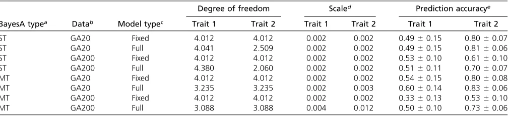
treated as unknowns. The conventional ST-BayesA model assumed the same prior for marker variance with v = 4.012 and s= 0.002 used in Meuwissenet al.(2001). For comparison, in conventional MT-BayesAvwas set to 4.012 andSto a diagonal matrix with 0.002 on the diagonal. For the two sets of simulated phenotypic traits controlled by 20 or 200 QTL, both conventional and full hierarchical ST-BayesA and MT-ST-BayesA were applied. Prediction accuracies were similar between conventional and full hierarchical models for the traits controlled by the 20 QTL genetic archi-tecture (Table 1). In contrast, for the traits controlled by 200 QTL, the full hierarchical models exhibited higher prediction accuracy for either one or both traits than the conventional BayesA methods for both ST- and MT-BayesA. For the low-heritability trait 1, the prediction accuracy (0.33) of MT-BayesA with fixed prior was significantly lower than the conventional ST-BayesA model. In contrast, the full hierar-chical MT-BayesA increased the prediction accuracy by 51% (from 0.33 to 0.50). A similar significant increase was ob-served for the high-heritability trait 2 (from 0.53 to 0.73). The different estimated priors for the marker variance in full hierarchical models (Table 1) compared to the conventional BayesA methods reflected the Bayesian learning process from the data. To take advantage of the full hierarchical ST- and MT-BayesA method, all BayesA analyses in all later sections of this study adopted the corresponding full hierar-chical models.
Prediction of breeding values using different ST- and MT-GS methods
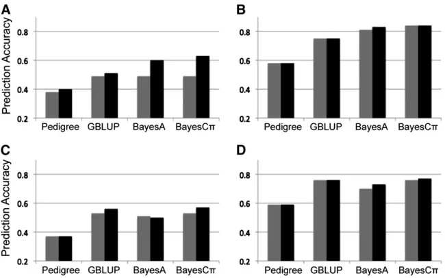
For comparison between the ST- and MT-GS methods, the simulated data sets with 20 QTL and 200 QTL were analyzed with four sets of ST- and MT-GS models: (1) pedigree-BLUP; (2) GBLUP based on SNP; (3) BayesA, and (4) BayesCp. In all cases, SNP-based genomic selection model performed better than pedigree-based BLUP method for both ST-GS and MT-GS methods for all simulated data (Figure 1). With 20 QTL (Figure 1, A and B), the prediction accuracies of low-heritability trait 1 increased 5, 4, 22, and Table 1 Prediction accuracies of conventional (fixed hyperparameter) and full-hierarchical BayesA methods for ST- and MT-GS models
Degree of freedom Scaled Prediction accuracye
BayesA typea Datab Model typec Trait 1 Trait 2 Trait 1 Trait 2 Trait 1 Trait 2
ST GA20 Fixed 4.012 4.012 0.002 0.002 0.4960.15 0.8060.07
ST GA20 Full 4.041 2.509 0.002 0.002 0.4960.15 0.8160.06
ST GA200 Fixed 4.012 4.012 0.002 0.002 0.5360.10 0.6160.10
ST GA200 Full 4.380 2.060 0.002 0.002 0.5160.11 0.7060.07
MT GA20 Fixed 4.012 4.012 0.002 0.002 0.5460.15 0.8060.08
MT GA20 Full 3.235 3.235 0.002 0.003 0.6060.14 0.8360.06
MT GA200 Fixed 4.012 4.012 0.002 0.002 0.3360.13 0.5360.10
MT GA200 Full 3.088 3.088 0.004 0.012 0.5060.10 0.7360.06
aST, single-trait BayesA; MT, multiple-trait BayesA.
bTwo data sets simulated for traits controlled by either 20 QTL (GA20) or 200 QTL (GA200). cFixed,fixed hyperparameter BayesA; Full, full hierarchical BayesA model.
36% using the MT-GS compared to ST-GS for pedigree-BLUP, Gpedigree-BLUP, BayesA, and BayesCp, respectively. In both ST- and MT-GS analysis, Bayesian methods outperformed both pedigree-BLUP and GBLUP with the 20 QTL scenario and BayesA was slightly better than BayesCp. For the high-heritability trait 2, the prediction accuracies of ST-GS and MT-GS were almost the same. In contrast, under the 200 QTL scenario (Figure 1, C and D), neither the ST or MT Bayesian methods outperformed GBLUP and within each type of method, the prediction accuracies between ST- and MT-GS were very similar.
Effect of heritability on predictions using multi-trait GS
Four combinations of trait heritability were simulated to test the effect of heritability on MT-GS accuracy. MT-BayesCp was used for this comparison. Under the ST-BayesCp anal-ysis, the prediction accuracy for the low-heritability trait (h2= 0.1) was 0.49. Given the genetic correlation of 0.5, the MT-BayesCpprediction accuracy of the low-heritability trait 1 was 0.67 and 0.70 when the heritability of correlated trait 2 was 0.5 and 0.8, respectively (Table 2). In contrast, the prediction accuracy for the medium- (h2= 0.5) or high-(h2= 0.8) heritability traits did not change as the heritabil-ity of the correlated trait changed.
Effect of genetic correlation between traits on the prediction of multi-trait GS
As genetic correlation increased between traits, the pre-diction accuracies increased for the low-heritability trait 1 (Figure 2). When the genetic correlation was 0.1 between the two traits, the prediction accuracy for the low-heritability trait was 0.63, which was already higher than the prediction accuracy based on the univariate analysis (0.49). As the genetic correlation increased, the prediction accuracies for the low-heritability trait also increased. In contrast, for the high-heritability trait 2, no obvious change in prediction accuracy was observed as the genetic correlation increased from 0.1 to 0.9.
Effect of error correlation between traits on the prediction of multi-trait GS
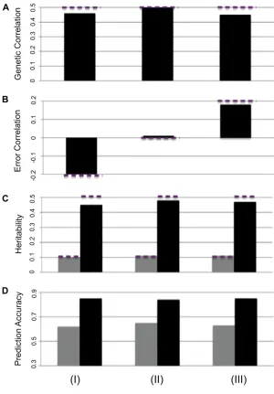
Phenotypic correlation between traits contains both genetic and error correlations. The error correlation under the de-fault simulation scenario was zero (Materials and Meth-ods). Three data sets were simulated with different error correlations (20.2, 0, and 0.2), while keeping other parameters at their default settings (Figure 3). The MT-GS model was able to separate error correlation from genetic correlation and estimate the heritability well. Furthermore, for both low- and high-heritability traits, the prediction accuracies were consistent across the three data sets.
Real pine breeding data analysis using multi-trait GS
The MT-GS models were applied to two disease-resistance traits in published pine breeding data (Resendeet al.2012) using a two-step analysis that reduced marker numbers by selecting on the rank of marker effect (see Materials and Methods) (Figure 4). Compared to prediction in the original publication (Resendeet al.2012), the ST-GS models in this study showed similar results for all models (GBLUP, BayesA, and BayesCp). This result suggests that the two-step analy-sis may be a useful variable selection method when millions of SNP markers from new sequencing technologies are used in genomic selection.
Figure 1Comparison of ST-GS (shaded) and MT-GS (solid) for correlated low-heritability (h2= 0.1) trait 1 (A and C) with high heritability (h2= 0.5) trait 2 (B and D) under the genetic architecture of 20 QTL (A and B) and 200 QTL (C and D). Genetic correlation between the two traits under each of genetic architectures is 0.5.
Table 2 Prediction accuracy for traits with different heritabilities
Heritability Prediction accuracya
Trait 1 Trait 2 Trait 1 Trait 2
0.1 0.5 0.6360.10 0.8660.05
0.1 0.8 0.7060.08 0.9460.02
0.5 0.8 0.8960.04 0.9360.03
0.8 0.8 0.9360.03 0.9460.03
The phenotype and genotype data used for ST-GS analysis were also fit with three MT-GS models. Within each of GBLUP, BayesA, and BayesCp, the MT-GS exhibited similar prediction capability to the ST-GS models (Figure 4). This
prediction pattern was similar to the pattern for the poly-genic genetic architecture in the simulation study. With MT-GS models it is also possible to predict a trait when individ-uals have been measured for other traits. For example, by setting each 10% of the Rust_gall_vol values to missing (similar to 10-fold cross-validation) and using both marker and Rust_bin data to predict these values, MT-BayesCphad a prediction accuracy of 0.48 (Figure 4), which was a 60% increase relative to the ST–GS method (0.30).
Discussion
Hyperprior optimization of Bayesian model for ST-GS and MT-GS methods
The conventional, fixed hyperparameter BayesA model allows locus-specific marker variances for markers in the model. This is a natural way to model the assumption that some markers are in strong LD with important QTL while others are not (Meuwissen et al. 2001). BayesA is easy to Figure 2 Effect of genetic correlation (x-axis) on the prediction accuracy
(y-axis) of low-heritability trait 1 (:) and high-heritability trait 2 (
•
) using MT-BayesCp.Figure 3 Effect of error correlation (20.2, 0, and 0.2 for
implement using conjugate priors through Gibbs sampling and has at times been shown, in both simulated and empir-ical data, to achieve higher prediction accuracy than ridge regression (Hayes et al.2010; Meuwissen et al. 2001). In BayesA, the hyperprior for the marker-specific variance is a scaled inverse-x2distribution with two parameters, degree of freedomn,and scales. Because most markers, in partic-ular SNPs, are biallelic, we estimate only a single marker-substitution effect per locus and the posterior and prior dis-tributions differ by only a single degree of freedom (Gianola
et al. 2009; although note that in the original publication, BayesA was applied not to biallelic markers but to multi-allelic marker haplotypes, Meuwissen et al. 2001). Conse-quently, the scale parametersin the prior has a strong effect on the shrinkage of marker effects. To address this draw-back, Habier et al.(2011) developed BayesDp that treated the scale parametersas a random variable to be estimated but still treated the degrees of freedom as known although this parameter strongly affects the shape of distribution. Thus BayesDp reduced the problems of BayesA but did not solve the dominance of the prior over the posterior distribution. Gianolaet al.(2009) suggested several possible solutions in-cluding development of a full hierarchical approach to esti-mating the optimal priors from the data instead of assigning
fixed values. In this study, both the degrees of freedom and the scale sparameter were given aflat prior and estimated using Metropolis sampling (Appendix). Under a simulated polygenic architecture, the full hierarchical BayesA model performed significantly better than the conventional fixed prior BayesA, and the difference was more important for multi- than single-trait analyses. Given that the genetic archi-tecture of traits of interest is unknown in practice use of the full hierarchical BayesA appears prudent.
Comparison of single-trait and multi-trait GS models
Daetwyler et al. (2010) investigated the impact of genetic architecture on the prediction accuracy of genomic selec-tion. They found that the GBLUP linear method showed relatively constant performance across different genetic architectures while the Bayesian variable selection method (BayesB) gave a higher accuracy compared to GBLUP when the traits were controlled by few QTL. This observation de-rived from simulation was also confirmed in real breeding data from different traits of Holstein cattle (Hayes et al.
2010). In a previous MT-GS study (Calus and Veerkamp 2011), different MT-GS methods were compared with each
other and with the corresponding ST-GS methods with sim-ulated data under a single genetic architecture. In our study, genetic architecture affected the relative superiority of MT-GS over ST-MT-GS. Under a major QTL genetic architecture, the Bayesian models performed better than GBLUP in both single-and multi-trait models, single-and the multi-trait analysis was strongly beneficial. Under the polygenic genetic architec-ture, however, GBLUP was equal to the Bayesian models and multi-trait analysis provided a slight improvement at best. This observation suggests that MT-GS can capture the genetic correlation between traits when major QTL are present more efficiently than when they are not. In addition, if other phenotypes are available on individuals that have missing data, phenotype imputation with MT-GS methods can be very useful (Calus and Veerkamp 2011), which was shown in the MT-BayesCpanalysis of real pine data.
Genetic correlation between traits is the basis for the be-nefit of MT-GS models. Among traits measured by breeders, not all traits are genetically correlated with other traits. For two traits simulated without genetic correlation, we found that MT-GS was inferior to ST-GS (data not shown). The decreased accuracy presumably arises because sampling leads to nonzero estimates of correlation in the training population and then to erroneous information sharing across traits in the validation population. To avoid the appli-cation of MT-GS on traits that are not genetically correlated, we can estimate that correlation between traits using the GEBVs derived from ST-GS models and apply MT-GS only where it is likely to be beneficial.
Low-heritability traits benefit from correlated high-heritability traits
Genetic correlation between traits has previously been exploited to improve the statistical power to detect QTL controlling traits of interest (Jiang and Zeng 1995; Fernie
et al.2004; Chesleret al.2005; Banerjeeet al.2008; Breitling
2010). It is important to note that MT-GS is modeled by directly taking advantage of such genetic correlation, whether it is favorable or unfavorable, and is not designed to break the undesirable genetic correlation.
Acknowledgments
We thank Mark Sorrells for valuable feedback on the manuscript. Partial funding for this research was provided by U.S. Department of Agriculture, National Institute of Food and Agriculture, Agriculture and Food Research Ini-tiative grants, award numbers 2009-65300-05661 and 2011-68002-30029.
Literature Cited
Banerjee, S., B. S. Yandell, and N. Yi, 2008 Bayesian quantitative trait loci mapping for multiple traits. Genetics 179: 2275–2289. Breitling, R., Y. Li, B. M. Tesson, J. Fu, C. Wu et al., 2008 Genetical genomics: spotlight on QTL hotspots. PLoS Genet. 4: e1000232.
Calus, M. P., and R. F. Veerkamp, 2011 Accuracy of multi-trait ge-nomic selection using different methods. Genet. Sel. Evol. 43: 26. Chen, Y., and T. Lubberstedt, 2010 Molecular basis of trait
corre-lations. Trends Plant Sci. 15: 454–461.
Chesler, E. J., L. Lu, S. Shou, Y. Qu, J. Guet al., 2005 Complex trait analysis of gene expression uncovers polygenic and pleio-tropic networks that modulate nervous system function. Nat. Genet. 37: 233–242.
Daetwyler, H. D., R. Pong-Wong, B. Villanueva, and J. A. Woolliams, 2010 The impact of genetic architecture on genome-wide eval-uation methods. Genetics 185: 1021–1031.
Fernie, A. R., R. N. Trethewey, A. J. Krotzky, and L. Willmitzer, 2004 Metabolite profiling: from diagnostics to systems biology. Nat. Rev. Mol. Cell Biol. 5: 763–769.
Gianola, D., G. de los Campos, W. G. Hill, E. Manfredi, and R. Fernando, 2009 Additive genetic variability and the Bayesian alphabet. Genetics 183: 347–363.
Gilmour, A. R., B. J. Gogel, B. R. Cullis, and R. Thompson, 2009 2009 ASReml User Guide, release 3.0. VSN Intl., Hemel Hempstead, UK.
Habier, D., R. L. Fernando, K. Kizilkaya, and D. J. Garrick, 2011 Extension of the Bayesian alphabet for genomic selec-tion. BMC Bioinformatics 12: 186.
Hayes, B. J., J. Pryce, A. J. Chamberlain, P. J. Bowman, and M. E. Goddard, 2010 Genetic architecture of complex traits and ac-curacy of genomic prediction: coat colour, milk-fat percentage, and type in Holstein cattle as contrasting model traits. PLoS Genet. 6: e1001139.
Jiang, C., and Z. B. Zeng, 1995 Multiple trait analysis of genetic mapping for quantitative trait loci. Genetics 140: 1111–1127. Liang, L., S. Zollner, and G. R. Abecasis, 2007 GENOME: a rapid
coalescent-based whole genome simulator. Bioinformatics 23: 1565–1567.
Meuwissen, T. H., B. J. Hayes, and M. E. Goddard, 2001 Predic-tion of total genetic value using genome-wide dense marker maps. Genetics 157: 1819–1829.
Resende, M. F. Jr., P. Munoz, M. D. Resende, D. J. Garrick, R. L. Fernandoet al., 2012 Accuracy of genomic selection methods in a standard data set of loblolly pine (Pinus taeda L.). Genetics 190: 1503–1510.
Xu, C., X. Wang, Z. Li, and S. Xu, 2009 Mapping QTL for multiple traits using Bayesian statistics. Genet. Res. 91: 23–37.
Xue, W., Y. Xing, X. Weng, Y. Zhao, W. Tanget al., 2008 Natural variation in Ghd7 is an important regulator of heading date and yield potential in rice. Nat. Genet. 40: 761–767.
Communicating editor: D. J. de Koning
Appendix
Metropolis Algorithm for Single-Trait BayesA Model
The joint posterior probability used for sampling the nandsparameters is
pðm;aj;s2j;s2e;n;syÞ ¼ P
n
i¼1pðyi
m;aj;s2
j;s2e;n;sÞ· P
p
j¼1pðaj
s2
jÞ· P p
j¼1pðs 2
jn;sÞ·pðn;sÞ;
Metropolis Algorithm for Multi-Trait BayesA Model
The joint posterior probability used for sampling the nandSm·mparameters is
pðm;aj;Saj;Se;n;Sm·myÞ ¼ P n
i¼1pðyi
m;aj;Saj;Se;n;Sm·mÞ· P
p
j¼1pðaj
Sa
jÞ · Pp
j¼1pðSajn;Sm·mÞ·pðn;Sm·mÞ;
wherepðyijm;aj;Saj;Se;n;Sm·mÞandpðajjSajÞwere multivariate (m·m) normal distributions,pðSajjn;Sm·mÞwas a scaled inverse Wishart distribution and pðn;Sm·mÞ was constant. The jumping distribution to sample the candidate ofn is the normal distribution with the existing value ofnas mean and variance equal to 0.2. The jumping distribution to sample the candidate scale matrixS*m·mwas scaled-inversed-Wishart(100,Sm·m).
Variable Selection Procedure and Posterior Distributions for Single-Trait BayesCp
The posterior distribution ofdjis
Prdj¼1 jy;m;a2j;d2js2a;s2e;p
¼ f
rjdj¼1;uj
ð12pÞ frjdj¼0;uj
pþfrjdj¼1;uj
ð12pÞ;
wherea2jandd2jare all marker effects and indicator variables except for markerj, respectively,rjequalsxjT(xjaj+e), andxj is the genotype vector for marker j.
In addition, fðrjjdj¼1;uj Þ is proportional to ðvdÞ21=2expð2r2jvd=2Þ, where vd can be two possible values, v0 or v1, depending whether the marker is in the model or not,
v0¼xTj xjs2e
v1¼ ðxjTxjÞ2s2aþxTj xjs2e:
Then if the Prðdj¼1jy;m;a2j;d2j;s2a;s2e;pÞis larger than the value sampled from a unit uniform distribution, the marker is included in the model. For markers in the model, the posterior distribution of marker effect,aj, is a normal distribution,
Nxj
y2x2ja2j
xjTxj=s2e þ1=s2a
·s2e
;xjTxj=s2e þ1=s2a
;
where x2janda2jare the marker genotype and effect excluding markerj,s2a, is the common variance shared by all the markers in the model. For the markers not in the model, the marker effect is equal to zero. The posterior distribution of overall population meanmand error variances2
e is the same as in ST-BayesA. Full conditional distributions used for Gibbs sampling for parameters were as follows.
For the common variance of marker effect,s2
a, a scaled inverse-x2distribution,
Ps2aa
¼inv-x2nþk;sþaTa
wheren, the degree of freedom in the prior, was assigned a value of 3,kis the number of markers included in the model, and
s, the scale parameter in the prior, is 0.01. For the probability of marker having a zero effect,p,a beta distribution:
pðpd;m;a;s2a;s2e;yÞ bðp2kþ1;kþ1Þ:
Variable Selection Procedure and Posterior Distributions for Multi-Trait BayesCp
The posterior distribution ofdjis similar to the ST-BayesCpexcept several parameters become matrices,
Prðdj¼1jy;m;a2j;d2j;Sa;Se;pÞ ¼
fðrjjdj¼1;uj Þð12pÞ
ðdetðvdÞÞ21=2exp
2rjvdrTj
2 ;
wherevdcan be two possible values,v0orv1, depending whether the marker is in the model,
v0¼xTjxjSe
v1¼ ðxTjxjÞ2SaþxTjxjSe:
The posterior distribution forp in MT-BayesCpis a beta distribution as in the ST-BayesCp. The prior ofSeand common variance–covariance across markers between traitsSawere inv-Wishart(n,Sm·m), wherenwas the number of traits plus 1 andSm·mis a diagonal matrix with size equal to number of traits and 0.01 on the diagonal. Full conditional distributions used for Gibbs sampling for parameters were as follows:
For the common variance of marker,Sa, a scaled inverse Wishart distribution
pðSajaÞ ¼inv-Wishart
nþk;Sm·mþaTa
;
wherekwas the number of markers in the model after the previous variable selection procedure andawas the matrix of estimated marker effects. For the error variance,Se, a scaled inverse Wishart distribution
pðSejeÞ ¼inv-Wishart
nþn;Sm·mþeTe
;
where nwas the number of individuals in the training population. Given the error varianceSe and marker effecta, the overall population mean vector is sampled from the multinormal distribution,
Nðy2Xa;Se=nÞ:
The posterior distribution forajis a multinormal distribution,
NððxTjxjS2e1þS2 1 a Þ2
1S21
e ðxTjðeþXa*jÞÞ T;ð
xTj xjS2e1þS2 1 g Þ2
GENETICS
Supporting Information
http://www.genetics.org/content/suppl/2012/10/11/genetics.112.144246.DC1
Multiple-Trait Genomic Selection Methods Increase
Genetic Value Prediction Accuracy
Yi Jia and Jean-Luc Jannink
File S1
Supporting Data
Genotype and phenotype data are available for download at