Application of Factor Analysis to k-means Clustering
Algorithm on Transportation Data
Sesham Anand
Department of CSE MVSR Engineering CollegeHyderabad
P Padmanabham, Ph.D
DirectorBharat Group of Institutions Hyderabad
A Govardhan, Ph.D
Professor, Dept of CSE,SIT, JNTU, Hyderabad
ABSTRACT
Factor Analysis is a very useful linear algebra technique used for dimensionality reduction. It is also used for data compression and visualization of high dimensional datasets. This technique tries to identify from among a large set of variables, a reduced set of components which summarizes the original data. This is done by identifying groups of variables which have a strong inter correlation. The original variables are transformed into a smaller set of components which have a strong linear correlation. Using several data analysis techniques like Principal Components Analysis (PCA), Factor Analysis, cluster analysis may give insight into the patterns present in the data but may also give different results. The aim of this work is to study the use of Factor Analysis (FA) in capturing the cluster structures from transportation (HIS) data. It is proposed to compare the clustering obtained from original data from that of factor scores. Steps involved in preprocessing the transportation data are also illustrated.
General Terms
Clustering, Preprocessing.
Keywords
Principal Components Analysis (PCA), Factor Analysis (FA), House Hold Interview Survey(HIS) Data, High Dimensional data.
1.
INTRODUCTION
Travel Demand Models are employed in decision making process of large infrastructure projects in Metropolitan cities. In this process, a number of traffic and transportation studies are conducted. Among them, the most expensive and challenging task is to estimate the travel patterns of passengers and good travel. The model is then based on the concept of travel making process. Home Interview surveys or origin based surveys are the most important surveys to capture travel patterns. Basically, it involves selecting a selected percentage of Households and then randomly selecting them for conducting interviews on Household members. The information is quite extensive and data can be considered are large. The usual procedure to employ data is to through standard statistical methods. The objective of this research is to employ data mining techniques so as to understand basic traits of the road users. This may help in better model development for subsequent analysis.
2.
HOME INTERVIEW SURVEY (HIS)
INFORMATION
A Home Interview survey among other surveys is the most important survey for any comprehensive transportation study. Representative samples of dwelling units are selected and
personal interviews are conducted to obtain travel characteristics for all members of the household by all modes of transportation on one full normal working day.
Vast amount of information is collected on various aspects of family structure, socio-economic characteristics, location of work/study places, and information of travel attributes by all trips made on that day.
This data is employed for analyzing existing travel patterns and behavior, to help in the calibration of Travel demand Models. These models are then employed to estimate and predict the future travel demand. Thus transportation demand and supply conditions can be critically examined and new facilities can be suggested.
2.1
Home Interview Survey Format
In the work, the data collected from Home Based Interviews as part of Transportation Planning studies of Hyderabad are utilized for analysis. The information provided is in three parts. The Home Interview Format was so designed that all these planning parameters are captured in a specially designed format by the study group. The format is broadly sub divided into three parts.
Page 1 A-GENERAL captures selected Household address and its location in the Traffic Analysis Zone, Total number of members, Type and Total number of Vehicles, Total household Income, Total expenditure on Transport by all members, whether the house is rented or own and whether they are happy about their stay in the locality and in the house.
Page 2 B-DETAILS OF EACH MEMBER OF HOUSE HOLD: Obtains details of each member of house, their relationship with the head of household particular regarding their age, gender, education level, occupation, income, type of vehicle they have, whether they use public transport and if so if they are a pass holder, and total money spent on transport etc.
Page 3 C-TRIP INFORMATION: Is designed to capture Travel Diary on one specific working day. This is designed to obtain all the components of travel in respect of Origin of trip ,Destination, Purpose of travel, details of access modes, line haul modes, cost and time invested, Parking charges, mode transfers are all gathered.
3.
PREPROCESSING OF DATA
over 100 variables some of which are described here (used in current work).
Filename: Household – A
1. FORM_NO This is the identification value for the form and also a particular household and is common for all the rest of the files. It has to be unique and cannot have negative values.
2. ZONE_NO, WARD_NO: These variables indicate the zone and ward in which the household resides. These variables will not contribute for further research and hence not included in further work.
3. MALES, FEMALES: These variables indicate the number of males and females in a house and hence cannot have negative values. They can have a zero value. It is assumed that a household cannot have more than 15 males or females and hence all values in these columns greater than 15 have been removed.
4. TOTAL_NO: This is an aggregate value based on the number of males and females. It cannot have negative values and has been checked. It is a summation of them. Hence it cannot have a zero value if there are values in MALES and FEMALES columns. It cannot have negative values and has been checked.
5. NO_MEM_STU: It indicates the number of members studying in the family.
6. VO_CY, VO_MOPED, VO_SCOOTER, VO_MOTORCY, VO_CAR: These variables indicate the number of bicycles, mopeds, scooters, motorcycles, cars owned by the family respectively. These variables cannot have negative values but can have missing values. All missing values are assumed to be as not an owner of the particular vehicle type.
7. VO_OTHERS: This variable value cannot be negative, but can have missing values. All missing values are assumed to be as not an owner of the particular data type.
8. TOTAL_VEHI: This variable is an aggregate value and is the summation of all vehicle type values. It cannot be negative nor has a zero value or missing values if there is a value in any of the vehicles columns. It has been checked.
9. MONTH_INCO: This variable has values which are in turn codes for the actual values. They are as follows:
Household Income Code in rupees. 1= 2500 6=20 000-25 000 2=2500-5000 7=25 000-30 000 3=5000-10 000 8=30 000-50 000 4=10 000 – 15 000 9 > 50 000 5=15 000-20 000
All values in the column have been replaced with the above values. All other values have been removed
10. MONTH_TRAN: It denotes the monthly expenditure for transport in the house hold. Many of the values in this column were 999. They have been removed. It has to have a value if there is a value in the corresponding column in the vehicle type and cannot be negative.
11. RESIDENCE: Residence of the household and is either owned or rented. It cannot have values other than 1 and 2, and cannot be negative.
12. LEVOFSAT_L, LEVOFSAT_R: These two variables indicate the level of satisfaction in the locality where the residence resides and residence itself. These variables were not considered in the present work.
Filename: Household B
13. FORM_NO: same as describe above, and must be any of the values as contained in Household -A file. As the values in the field are unique to some extent and repeated many times, this variable may not influence the model to be created. Hence this variable has been removed
14. ZONE_NO: It has been assumed that this variable will not influence the behavior or characteristics of the household or its members. Also its values are very less and repeating for many rows. Hence it has been removed from the dataset. 15. PERSON_NO: This indicates family persons in a house. It is assumed that it is not of much significance to the actual outcome. So this variable has been ignored.
16. REL_HEAD: It indicates the relation of a person in the family w.r.t the family head. The family head corresponds to value ‘1’ and the interest is only in family head and earner. All other rows with values other than ‘1’ have been removed. 17. AGE: Corresponds to age of a member in the family. These values cannot be negative and cannot be more than 100 and zero. Many rows had age value as zero and more than 100. They had been removed.
18. SEX: Indicates the sex of a person. It can be either male or female i.e. 1 or 0 only. It cannot be left blank nor have any other values.
19. EDUCATION: It reflects the education level of a person ranging from illiterate to post graduate. It cannot be more than 5 and less than 1.
20. OCCU_CODE: It is the occupation of a family member and values range from 1 to 11.
21. OCCU_ORGAN: It is the location of the organization in which a person works. It has not been included in the current research.
22. INCOME: This variable indicates the monthly income of a person in the family. All the rows having zero income or negative or any invalid number like 999 have been removed from the dataset. Persons of no income are of no significance for the research and hence have been removed. 23. VO_CODE: Indicates the vehicle ownership, and is not considered for further analysis.
24. VO_NUMBER: Indicates the number of vehicles a person has and is not considered for further analysis.
25. RAIL_BUS_P: Indicates whether a person holds a railway or bus pass. It has to be 0, 1 or 2 only.
26. PASS_COST: Cannot be negative or illegal values like 999. In that case they have been removed
4.
BACKGROUND
The present work is largely based on a similar work done by Combes and Azema [1] wherein principal components analysis was used to propose a new algorithm on elderly people-disability data. Anasuya and Latha [2] applied PCA based k-means algorithm on various UCI datasets and showed that it performs better compared to conventional k-means algorithm. Prabhu P, Anbazhagan [3] showed that by reducing the data using PCA showed significant improvement in clustering. Chris and Xiaofeng [4] applied PCA on gene data and internet newsgroup data and showed the benefits of applying PCA. Indhumathi and Sathiyabama [5] developed a new algorithm bisecting k-means using PCA on k-means algorithm. Napolean and Pavalakodi [6] used dimensionality reduction method PCA on breast cancer data and showed the improvement achieved over conventional data. Previous work of the authors [7] involved clustering on original data. To the knowledge of the authors, no work exists on applying PCA or factor analysis (FA) on Transportation data. This paper applies FA on the dataset and uses it to apply k-means algorithm and illustrate the results.
5.
ANALYSIS
The collected data has been subjected to correlation analysis and it was found that majority of the variables are correlated with correlation coefficient greater than 0.3 or greater. The communalities are found to be significantly higher.
5.1
Principal Components Analysis
The HIS dataset has more than 140 variables and it is difficult to visualize them and find out their associations. PCA [8] is one way of re-expressing the data and allows reorienting the data so that the first few dimensions give the maximum information possible. All the principal components are uncorrelated with all others. Each principal component is a linear combination of all the original variables. The first component exhibits the maximum variance and so on. PCA is primarily used in the present work for dimension reduction. Little redundancy was observed in the dataset. Working with fewer variables enables for easier visualization and identifying interesting patterns.
Let be the matrix [8] of original variables in the dataset. Let ,
etc. be unit vectors oriented along the ellipsoidal axes and are perpendicular to each other. Let
, ), etc. be the new transformed variables. Now , where X is an n x 3 matrix whose elements are the values X1,X2,X3 etc. Z1 is the
variance accounted for by the first principal component, Z2 is
the variance accounted for by the second principal component not already accounted for by the Z1 etc., i.e.
. The greater this value the more information from the original data is contained in these components although the variance accounted for by Z2 is smaller than Z1 and so on.
Hence the transformation rotates the axes of the original data while preserving their orthogonality. Relationship between Z and original variables X is illustrated with a correlation matrix and are called principal component loadings and they help in interpreting the principal components and how much of variance in each original variable X is accounted for by the principal components.
is called as the eigenvalue-eigenvector problem. Here u is called as eigenvector and λ is called as eigenvalue. The solution to PCA consists of p positive eigenvalues and associated eigenvectors. PCA can be
performed either by eigenvalues analysis of correlation matrix R or singular value decomposition of X.
5.2
Factor Analysis
Factor Analysis (FA) [8] is also known as exploratory factor analysis. This technique is also used for dimensionality reduction and finding association between variables as PCA but the difference is that it is based on common factor model. The common factor model assumes that the observed variance in variables is attributed to a small number of common factors and a single specific factor. Ultimately the objective is to identify the common factors and identify the relationship with observed data. For the HIS data the aim is to identify the source of common variance underlying the questionnaire used to collect data.
Let ξ1, ξ2, … ξi be a set of common factors [8] and δi be the
specific factor. Let X be set of observed variables. All the specific factors are mutually uncorrelated. In general a c factor model can be represented as follows [8]
Where λ represents the extent to which each measure X reflects the underlying common factor ξ. Hence the variance of Xi is
Here λi2 is called the communality of Xi. the relation between
the observed variables and the factors is called as factor loadings. The orientation of the axes representing the common factors can be changed which will change the factor loadings.
5.2.1
Kaiser’s Varimax Rotation
In the current work, Kaiser’s Varimax Rotation [8] has been used in FA. Since the common factors are uncorrelated, the total variance of all common factors is given by the sum of squared loadings i.e. whereaik is the correlation
between variable I and common factor k. the aim is to find a rotation so that a2ik are close to 1 or zero. The varimax
procedure chooses a rotation matric T to maximize the total column variance of a2ik. The kth column variance is given by
Maximizing the sum of these column variances Vk for all
factors k is nothing but maximizing the following expression
The location of each of the original observations in the reduced factor space is called factor scores.
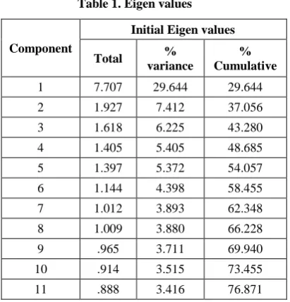
Table 1. Eigen values
Component
Initial Eigen values
Total %
variance
% Cumulative
1 7.707 29.644 29.644
2 1.927 7.412 37.056
3 1.618 6.225 43.280
4 1.405 5.405 48.685
5 1.397 5.372 54.057
6 1.144 4.398 58.455
7 1.012 3.893 62.348
8 1.009 3.880 66.228
9 .965 3.711 69.940
10 .914 3.515 73.455
11 .888 3.416 76.871 Fig 1: Screen Plot showing components with Eigen values
Table 2. Rotated Component matrix
Component
Pro
sper
ity
H
o
u
se
h
o
ld
S
tr
u
ctu
re
Ba
sic
Ve
h
icle
O
wner
shi
p
Ca
r
O
wner
shi
p
Av
a
il
a
b
il
it
y
o
f
Pa
rk
in
g
Pu
b
li
c
Tr
a
n
spo
rt
O
cc
u
p
a
tio
n
Pu
rp
o
se
o
f
Tr
a
v
el
Tr
a
v
el
Ex
p
en
d
it
u
re
Ac
ce
ss
to
O
wn
Ve
h
icle
Pa
rk
in
g
Co
st
MALES .370 .529 .317
FEMALES .417 .696
TOTAL_NO .487 .755
NO_MEM_STU .810 .258
VO_CY .848
TWO_WHLR .393 .689
VO_CAR .843
TOTAL_VEHI .694 .513
MONTH_INCO .473 .647
a_MONTH_TRAN .649 .510
RESIDENCE .818
AGE .533 .320 .366
SEX .784
EDUCATION .282 .760
OCCU_CODE .323 .270 -.320 .637
INCOME .859
VO_CODE .992
RAIL_BUS_P .879
DISTANCE -.324 .780
PURPOSE -.853
S1_DISTANC -.439 -.270 .326 .354
S1_MODE .708 .310
S1_TRA_TI -.644 -.366
S1_TYPE_PA .817
S1_COST_PA .994
[image:4.595.323.541.78.268.2] [image:4.595.70.533.340.754.2]5.3
Factor Analysis vs. Principal
Components
The essential technical difference between factor analysis and principal components analysis [9] is that in principal components analysis, when analyzing the correlation matrix, we insert communality estimates of 1.0 in the diagonal of the matrix. That is, in solving for the Eigen values and eigenvectors of the correlation matrix, it is assumed that the communality is 1.0 for each pair of variables. In factor analysis on the other hand, the communalities are not assumed to be 1.0. Rather, the communalities are estimated, and are inserted into the diagonal before solving for the relevant Eigen values and Eigen vectors. That is the main technical (not theoretical) difference between principal components analysis and factor analysis. In short, principal components analysis analyzes the total variance in the data set, whereas factor analysis focuses on the variance that is common to the variables
Communalities for all the variables were high. This is the proportion of each variable's variance that can be explained by the factors. The number of factors selected was 11 as the intended variance to be explained by them was fixed at 75%. Looking at the screen plot in Fig: 1 also confirms the selection of the number of components.
Based on the high factor loadings seen from the Table 2 for different variables, the factors are given proper names.
5.4
Cluster Interpretation on Factors
Author’s previous work [7, 10, 11] involved clustering on original Transportation Data and proper interpretation of clusters was made. Now, an attempt is made to do the same on factors obtained as follows.Cluster 1: This cluster has average values of household prosperity, with medium sized family structure. These families owned few cars and other vehicles and they are using parking facilities a lot. Majority of these families used public transport, high occupation
Cluster 2: This cluster illustrates less income or low prosperity household, with high family structure. Obviously they owned very few vehicles and in turn parking facilities. Surprisingly they even are using public transport. Since occupation is high majority of them might be laborers or working in the agriculture field.
Cluster 3: This cluster shows families with less prosperity, average size of families, minimum vehicle ownership etc. Basically it reflects middle class family households.
Cluster 4: This cluster reflects high prosperity households, medium sized families, more car or vehicle ownership, less parking usage and less usage of public transport. Basically this group reflects high income families.
As seen here, the grouping seems to be much clear when compared to clusters from original data.
6.
COMPARISON
K-means algorithm is applied on the original data and on all 26 factor solutions and the results are shown in Table 3.
6.1
Results
[image:5.595.317.540.308.460.2]K-means algorithm was applied on the original data and on 11 factor scores and results are shown in Table 4.
Table 3. K-means applied on original data and all factors
Data SSE Time(seconds)
Original Data 624.5 0.36
Factors(26) 94.65 0.14
Table 4. Log-likelihood comparison
Data Log Likelihood Training Time(seconds)
Original Data -20.54 0.24 Factors (11) -19.74 0.40
Looking at Table 4, it is noticed that the algorithm fared better on factors.
As the Table 3 suggests, clustering factors gave the least error. Based on the experiments conducted, it is suggested to recommend a series of steps for analyzing HIS transportation data. The preprocessing to be done is illustrated in Fig: 2.
Fig 2: Visualization of original raw data
Fig 3: Visualization of Factors obtained by Factor Analysis
6.2
Recommendations
[image:5.595.317.540.496.637.2]this, it is proposed to explore the use of factor analysis in cluster analysis for given data..
Fig 4: Preprocessing steps
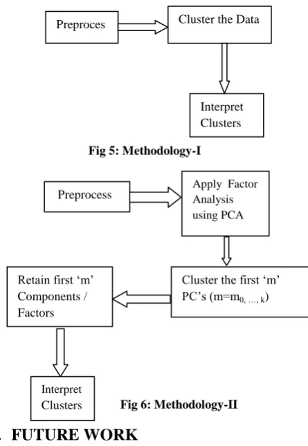
[image:6.595.315.545.77.219.2]Firstly, clustering was done on normal data (Fig: 5) and appropriate parameters were noted. Then, factor analysis was done on the data and 11 factors were identified and appropriately named. Clustering was then done on the factors alone (Fig: 6) and then a comparison done. It is noted that the error got reduced significantly when factors were used. The clusters were also easily interpretable. The figure shows the two methodologies adopted and the recommendation is to use methodology II.
Fig 5: Methodology-I
Fig 6: Methodology-II
7.
FUTURE WORK
As an extension to the current research, other partitional clustering algorithms can also be applied. Also, it is proposed to do an extensive comparison of cluster validity indices on the data and suggest an appropriate validity measure. Similarly, as is widely known, the effect of distance measures used by partitional clustering algorithms will be studied.
[image:6.595.55.284.98.239.2]Fig 7: Proposed Future work
Fig: 7 shows the future direction of research to be taken up by the authors.
8.
CONCLUSION
In this work, the transportation data was preprocessed and details were illustrated. The data was clustered by applying a clustering algorithm k-means on the data set. Then, Factor Analysis was applied on the original data and then the same clustering algorithm is applied on the factor scores obtained. A comparison of the effectiveness of clustering on the original data with that on the factor scores has been presented and is found to be useful. Finally appropriate recommendations have been made and future work illustrated.
9.
REFERENCES
[1] Indumathi R, Dr. Sathiyabama S, Reducing and Clustering high Dimensional Data through Principal Component Analysis, International Journal of Computer Applications (0975 – 8887)Volume 11– No.8, December 2010.
[2] Chris Ding, Xiaofeng He, k-means clustering via principal component analysis, Proceedings of the 21st International Conference on Machine Learning, Banff, Canada, 2004.
[3] Sesham Anand, Sai Hanuman A, Dr. Govardhan A, and Dr. Padmanabham P, Application of Data Mining Techniques to Transportation Demand Modelling Using Home Interview Survey Data, International Conference on Systemics, Cybernetics and Informatics 2008. [4] Sesham Anand, Dr P. Padmanabham, Dr. A Govardhan,
Dr. A. Sai Hanuman, Performance of Clustering Algorithms on Home Interview Survey Data Employed for Travel Demand Estimation, International Journal of Computer Science and Information Technologies, Vol. 5 (3) , 2014, 2767-2771
[5] Indhumathi R, Dr. Sathiyabama S, Reducing and Clustering High Dimensional Data through Principal Component Analysis, International Journal of Computer Applications (0975 – 8887)Volume 11– No.8, December 2010
[6] Napolean D, Pavalakodi S, A New Method for Dimensionality Reduction using KMeans Clustering Algorithm for High Dimensional Data Set, International Journal of Computer Applications (0975 – 8887) Volume 13– No.7, January 2011
[7] Sesham Anand, Dr P. Padmanabham, Dr. A Govardhan, Dr. A. Sai Hanuman, Performance of Clustering Preproces
s
Cluster the Data
Interpret Clusters
Preprocess Apply Factor Analysis using PCA
Retain first ‘m’ Components / Factors
Cluster the first ‘m’ PC’s (m=m0, …, k)
Interpret Clusters
Preprocessing
Replace missing values, Identify outliers, Schema Integration, removing useless attributes according to domain knowledge, remove redundant attributes
Cleaned Data
Obtained Clusters
Compare the cluster results using cluster validity measures
[image:6.595.62.285.356.679.2]
Algorithms on Home Interview Survey Data Employed for Travel Demand Estimation, International Journal of Computer Science and Information Technologies, Vol. 5 (3) , 2014, 2767-2771
[8] James Lattin, J. Douglas Carrol, Paul E. Green, Analyzing Multivariate Data, 2004, Thomson Learning, Shroff Publishers, ISBN: 981-243-514-X
[9] Data & Decision (2009) - Factor Analysis II Daniel J. Denis, Ph.D., University of Montana, http://psychweb.psy.umt.edu/denis/datadecision/factor/d d_fa_part_2_aug_2009.pdf
[10] Sesham Anand, Sai Hanuman A, Dr. Govardhan A, and Dr. Padmanabham P, Application of Data Mining Techniques to Transportation Demand Modelling Using Home Interview Survey Data, International Conference on Systemics, Cybernetics and Informatics 2008. [11] Sesham Anand, Sai Hanuman A, Dr. Govardhan A, and