Blind image separation using pyramid technique

(1)

R E S E A R C H

Open Access

Blind image separation using pyramid

technique

M. Y. Abbass

1,2

and HyungWon Kim

1*

Abstract

Signal and image separation is an important processing step for accurate image reconstruction, which is

increasingly applied to many medical imaging applications and communication systems. Most of the conventional separation approaches are based on frequency domain and time domain. These approaches, however, are sensitive to noise and thus often produce undesirable results.

In this paper, we propose a novel method of image separation. It incorporates the property of pyramid component extracted from the image and a finite ridgelet transform (FRT) to obtain a precise analysis of the images and thus correctly separate the images even in a highly noisy environment. We obtain the multiple components of the target images by employing a pyramid processing, which operates in the various domains and thus can decompose the image into multiple components.

In addition, the pyramid decomposition in the proposed method can eliminate information redundancy in the target image and thus can substantially enhance the quality of image separation. We have conducted extensive simulations, which demonstrate that the proposed pyramid structure with FRT outperforms the conventional methods based on time domain and trigonometric transforms.

Keywords:Pyramid technique, Finite ridgelet transform (FRT), ICA, Blind source separation (BSS), Pyramid technique

1 Introduction

Blind source separation (BSS) has been one of the major research areas for over a decade and is receiving growing attention due to its processing applications in image and signal processing. It aims at extracting a set of source signals from an observed mixture of signals with little or no information about either the mixing environment or the mixing process and sources. The applications of BSS range from medical engineering to neuroscience and also from telecommunications to financial time series analysis. For example, its recent applications include astronomical imaging, remote sensing, medical imaging, biological data analysis, image and speech signal pro-cessing, etc. [1–3].

Independent component analysis (ICA) has been often regarded as an attractive solution to the BSS problem. Its process is based on non-Gaussianity method, and so, it can utilize its statistical independence of the sources to calculate

the de-mixing matrix and extract the source signals with a scaling factor and permutation [4,5].

In biomedical applications, ICA has been applied to the functional magnetic resonance imaging (fMRI) data ana-lysis applies ICA. For example, in the article of [6], tem-poral dynamics and their spatial sources have been successfully recognized by real-valued ICA. In addition, the ICA has been applied to [7] for classification in elec-troencephalography (EEG) which has a two-state output (fatigue state vs. alert state). ICA has been also used in gait activity analysis, which usually relies on multiple sensors such as pressure, gyroscope, and accelerometer. The mul-tiple sensors often incur crosstalk problem sensors where each sensor interferes with another sensor. ICA has also been exploited in [8] to enhance an automated classifica-tion technique to recognize toe walking gait from normal gait in idiopathic toe walking (ITW) children.

The simplest BSS model assumes the existence ofn in-dependent sources s1, s2,..., sn, and the same number of linear and instantaneous mixtures of these sources, x1, x2,...,xn, that is,

* Correspondence:[email protected]

1_{Department of Electronic Engineering, College of Electrical and Computer}

Engineering, Chungbuk National University, Cheongju City, South Korea Full list of author information is available at the end of the article

(2)

xj¼aj1s1þaj2s2þ:…þajNsN; 1≤j≤N ð1Þ In vector-matrix notation, the above mixing model in the presence of noise can be expressed as

x¼Asþn ð2Þ

Here,Ais anN×Nsquare mixing matrix.

Equation (2) can be expressed in matrix form as follows:

x1ð Þk ⋮ xNð Þk

0 @

1 A¼ A

T

11 ⋯ AT1N

⋮ ⋱ ⋮

AT

N1 ⋯ ATNN

0 @

1 A s1ð Þ_⋮k

sNð Þk

0 @

1

Aþ n1ð Þ⋮k nNð Þk

0 @

1 A _ð3Þ

The model described above is represented in Fig.1. The de-mixing process [9–11] can be represented by calculating the separating matrixW, which is the inverse of the mixing matrix _A, and computing the independent sources, which are obtained by

s¼Wx ð4Þ

In this paper, we introduce a novel (differential) image separation algorithm that separates mixed images by extracting the components of the images using a pyra-mid technique. In this way, the image structure can be decomposed into multiple images of different scales. The proposed method creates different levels of scaled-down images in a pyramid structure. We there-fore conduct the separation process on each level of the pyramid. While the lowest scale image at the top of the pyramid has same features, it incurs lower redundancy than the original image at the bottom of the pyramid. Our separation process conducted on the scaled images of the pyramid can, therefore, lead to better separation performance with lower redundancy in the resulting sep-arated images.

Our method has the following two advantages over the most of ICA methods. Its first advantage is the high performance under noisy condition. Most of the ICA techniques consider only noiseless data; hence, they often lead to poor results in the presence of noise [12, 13]. In contrast, our method can separate the mixed image under a noisy condition and still provide high peak signal-to-noise ratio (PSNR). The second advantage is its fast processing and yet accurate separation results. Since it removes the redundancy in the image informa-tion, it can obtain the estimated image sources faster and more accurately than the ICA methods. The key contribution of proposed algorithm extracts the scaled-down images of the pyramid, in a way that

Fig. 1The mixing and de-mixing models

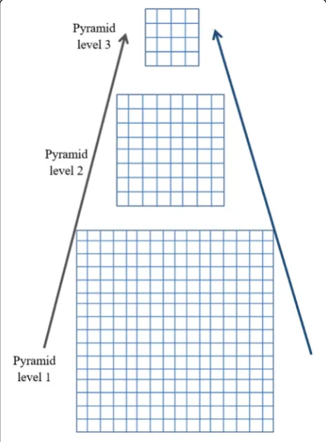
Fig. 2Pyramid technique effect

(3)

maintains the important information of the original image, while reducing the redundant information.

The remainder of this paper is organized as follows. In Section 2, we provide the related work. Section 3 illus-trates various techniques including the principle of pyra-mid image, finite ridgelet transform, and trigonometric transforms. In Section 4, the proposed image separation approach is presented. To demonstrate the effectiveness of the proposed technique, an extensive set of simulation experiments and performance comparison is reported in Section 5. Finally, Section 6 presents the concluding remarks.

2 Related work

In literature, there have been several papers published, which propose various approaches to the source image separation problem. The method in [14] considers a nonlinear real-life mixture of document images that occur when a page of a document is scanned and the back page shows through. It used a separation method based on the fact that the high-frequency components of the images are sparse and are stronger on one side of the paper than on the other one. Astrophysical image separation has been considered for a blind source separ-ation method in [15]. In the work of [16], feedback sparse component analysis of image mixture was devel-oped to extract the image sources by utilizing a feedback

mechanism and sparse component analysis (SCA). In [17], a wavelet packet transform method was proposed in combination with a geometric de-mixing algorithm. It decomposes the mixed images by a wavelet transform (WT) and then uses the most relevant component as an input to its de-mixing geometric algorithm.

In the article of [18], columns or rows of mixed images were concatenated to arrange them into a 1-D mixed image. Then, a source separation of frequency-time ap-proach with mutual diagonal was introduced to enhance these 1-D signals to resolve their components. Then, two-dimensional (2-D) astrophysical image components were achieved by segmenting separated 1-D original sig-nals and rearranging these segments as columns or rows. Recently, researchers implemented sparse component analysis (SCA) to improve the method of blind image separation [19, 20]. These approaches could accurately separate the image mixtures using linear clustering when the linear clustering has less run time than super-plane clustering techniques, and the image sources are sparse enough [21].

The work of [22] applied the discrete cosine transform (DCT) as an approach to get the information in the fre-quency domain. It uses a block-segmented DCT reorganization to get the information in the segmented blocks while selecting the sparsest block by comparing the linear strength in each block. Moreover, the authors

(4)

of [22] used the geometric characteristic of sparse blocks to study the linear orientations that match with the mix-ing matrix columns.

3 Methods of the proposed scheme

3.1 Principle of pyramid image enhancement

An image can be decomposed and analyzed in a form of a pyramid with a few levels of scaled-down images. The pyramid places the original image at the first level and adds scaled-down images at the higher levels [23] as il-lustrated in Fig.2.

The pyramid scales down an image using the low-pass filter with a Gaussian mask expressed by Eq.5.

H¼ 1

256

1 4 6 4 1

4 16 24 16 4

6 24 36 24 6

4 16 24 16 4

1 4 6 4 1

0 B B B B @

1 C C C C A ð5Þ

The motivation behind our pyramid technique is that the surrounding pixels within a certain area often have the similar characteristics, and thus, they are highly correlated with each other. To estimate the inverse matrix from Eq. (4) directly, the mixed image is converted from 2-D sig-nal to 1-D sigsig-nal. It is, therefore, inefficient to apply ICA

algorithm to the pixel values, since most of the information around neighboring pixels is redundant, and the entropy of the pixels in the same area is low. Therefore, as a more effi-cient method to calculate the inverse matrix, we proposed a new technique that can remove the redundancy without af-fecting the information, and that can increase the entropy, while maintaining the features. The pyramid technique has been proposed in this paper, which scales down the image while maintaining the main features such as salient features and removing the redundant information. In the presented work, we use three levels to construct pyramid levels as shown in Fig. 2. Level 1 is the input image. Level 2 is the output after applying the filter based on Eq. (5), followed by a downsampling step. The above steps are then repeated to produce level 3. The ratio between the image outputs of the two consecutive levels determines the scale of the pyra-mid levels with respect to the original image. We can use these scales for further processing using ICA separation.

3.2 Transform techniques

3.2.1 Ridgelet transform

Ridgelet transform (RT) is a highly effective approxima-tion approach to represent an image object as described by Candes and Donoho [24, 25]. It has a discontinuity across a line, and a curvelet, which is adopted in their pa-pers as a type of RT, and is an effective transform for

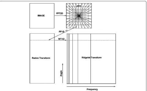
Fig. 4Ridgelet transform flowchart

(5)

objects with discontinuities across curves. The approxima-tion quality of RT is very close to the ideal Lagrangian con-dition and is in general better than any other algorithms such as Fourier transform (FT) and wavelet transform (WT). Due to such advantage, RT is widely used in image analysis, such as watermarking, image enhancement, image de-noising, and texture classification [26,27].

Suppose that there is a functionψ:R→Rsatisfying the admissibility condition

Z

R ^

ψ ξð Þ

j j2₌_{j j}_ξ2_dξ_<_∞ ð₆Þ

whereψ^ stands for the Fourier transform of the function

ψ. For eacha> 0, b ∈R, and θ∈ [0, 2π], a bivariate RT

ψa,b,θ:R2→R2is defined as

ψ_a_;_b_;θðx1;x2Þ ¼a−1=2:ψððx1 cosθþx2 sinθ−bÞ=aÞ ð7Þ

For a fixed θ, ψa, b, θ(x1,x2) is constant along the line x1cosθ+x2sinθ= constant.

Given an integrable signal f(x1, x2), the RT is defined

as

RTfða;b;θÞ ¼

Z

R2f xð 1;x2Þψa;b;θðx1;x2Þdx1dx2 ð8Þ

It follows that

ψa;b;θðx1;x2Þ ¼ Z

R2ψa;bð Þt δ x1

cosθþx2 sinθ−t

ð Þdt

ð9Þ

whereψa,b(t) =a−1/2.ψ((t−b)/a). Then the RT can be expressed as

RTfða;b;θÞ ¼ Z

R2ψa;bð Þt Z

R2f xð 1;x2Þδðx1cosθþx2sinθ−tÞdx1dx2dt ¼

Z

R

ψa;bð ÞtRfðθ;tÞdt

ð10Þ

As a result, the formula is represented by (a)

(b)

(c)

(6)

R_fðθ;tÞ ¼

Z

R2f xð 1;x2Þδ x1

cosθþx2 sinθ−t

ð Þdx1dx2

ð11Þ

From signalf(x1,x2), we can calculate Radon transform

(RAT). Thus, the RT space can be expressed as an im-plementation of a 1-D wavelet transform to the slices of the Radon space.

It is known that approximate RAT for an image can be effectively computed with the fast Fourier transform (FFT). This approach is summarized by [28–30]:

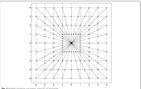
(a) 2-D FFT step: calculate the 2-D FFT of the image. (b) Cartesian to polar conversion step: obtain samples

on the recto polar as shown in Fig.3.

(c) 1-D inverse FFT step: calculate the 1-D inverse FFT on each angular line.

For the implementation of the Cartesian to polar con-version, we use a rectopolar coordinate plane. The geometry of this coordinate plane is presented in Fig.3, where the data points are marked with circles. Here, for an image of size n ×n, there are 2n radial lines in the frequency plane selected by connecting the origin to the vertices lying on the boundary of the array. The grid lines of the rectopolar coordinate plane are the intersec-tions between the set of radial lines and that of Cartesian lines parallel to the axes. Thus, there are 2n ×n points (marked with circles) on the rectopolar grid lines, and the corresponding data structure is a rectangular format withn× 2nelements.

To complete the RT, we perform a 1-D wavelet trans-form along the radial variable in Radon space. Figure 4 displays the flow graph of the RT.

Do and Vetterli supposed a different execution of the ridgelet transform called finite ridgelet transform.

It has numerical exactness like the RT with little com-putational complications. As supposed above, a separate RT can be realized via a Radon transform and a 1-D discrete wavelet transform (DWT) as presented in Fig.4. The finite Radon transform (FRAT) is simply an addition of image pixels over a certain set of lines. Those lines are known in a limited geometry in a similar scheme to the lines for the constant Radon transform (RAT) in the Euclidean geometry [12–16].

We denote Zp= {0, 1, 2 ... p−1}, where p is a prime number. Note that Zp is a limited field with modulo p processes.

Then, the FRAT of a real function f on the limited grid Zp

2

is given by

rkb c ¼l FRATfðk;lÞ ¼ 1= ffiffiffip p

X

i;j ð ÞεLK;i

f ið Þ;j ð12Þ

Here, Lk,l denotes the group of points that make up a

line on the latticeZp2.

Lk;l¼ ð Þi;j :j¼kiþlðmodpÞ; i ∈Zp

;0≤k≤p−1

i;j ð Þ:j∈Zp

;k¼p

ð13Þ

The lines of the FRAT show a wrap-around effect in the transform. This means that the FRAT deals with the input image as one period of a periodic picture. In the

Fig. 6Block diagram of the proposed image separation algorithm

(7)

FRAT domain, the energy is best compressed if the mean is removed from the image f(i, j) prior to the transform.

In Eq. (12), the factor 1=pffiffiffip is supplied in order to normalizel2standard between the result and input of the

FRAT. With an invertible FRAT and by using Eq. (13), we can have an invertible separate finite ridgelet transform (FRT) by taking the separate wavelet transform on each repetition of FRAT projection repetition, (rk[0],rk [1],…

rk[p−1]), where the trendkis constant. The total record-ing is known as the FRT as shown in Fig.4.

3.2.2 Discrete wavelet transform

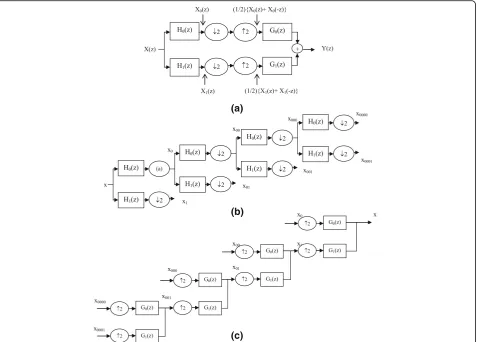
Wavelets have become an efficient tool in several signal processing areas such as signal de-noising, image fusion, and signal restoration and compression. The conven-tional discrete wavelet transform (DWT) may be regarded as the result of filtering the input signal with a bank of band-pass filters whose impulse responses are all approximately given by scaled versions of a mother wavelet. The scaling factor between adjacent filters is usually 2:1, which leads to octave bandwidths and center frequencies that are one octave apart from each other as illustrated by Fig. 5 [31]. The outputs of the filters are usually maximally decimated so that the number of DWT output samples equals the number of input sam-ples and the transform is invertible as shown in Fig.5.

The art of calculating a good wavelet lies in the design of appropriate filters,H1,H0,G1, andG0, to realize

vari-ous trade-offs between frequency and spatial space char-acteristics while satisfying the condition of perfect reconstruction (PR) introduced by [31]. In Fig. 5, the procedure of interpolation and decimation by 2:1 as the result ofH1andH0defines all odd components of these

signals to zero.

For the low pass branch, this is equivalent to multiply-ingx0(n) by1₂ð1þ ð−1ÞnÞ.

Hence, X0(z) is converted to1₂fX0ðzÞ þX0ð−zÞg.

Simi-larly,X1(z) is converted to1₂fX1ðzÞ þX1ð−zÞg.

Thus, the expression for_Y(_z) is given by the equation below [31]:

Y zð Þ ¼1

2fX0ð Þ þz X0ð Þ−zgG0ð Þz

þ1

2fX1ð Þ þz X1ð Þ−zgG1ð Þz

¼1 2X zð Þ

H0ð ÞzG0ð Þz þH1ð ÞzG1ð Þz

þ1 2Xð Þ−z

H0ð Þ−zG0ð Þz þH1ð Þ−zG1ð Þz

ð14Þ

The first PR condition requires aliasing cancelation and forces the above term inX(−z) to be zero [31].

Hence, {H0(−z)G0(z) +H1(−z)G1(z)} = 0, which can be

achieved if:

H1ð Þ ¼z z−kG0ð Þ−z andG1ð Þ ¼z zkH0ð Þ−z ð15Þ Here,kis limited to odd numbers (usuallyk= ± 1). From X(z) to Y(z), the transfer function need to be unity in the second condition of PR:

Fig. 7Flowchart of the FastICA algorithm

(8)

H0ð ÞzG0ð Þ þz H1ð ÞzG1ð Þz

f g ¼2 ð16Þ

3.2.3 Trigonometric transform

The two primary trigonometric transforms are the discrete cosine transform (DCT) and the discrete sine transform (DST). Trigonometric transform has an energy compaction feature. The properties of these transforms are described below.

3.2.3.1 DCT The DCT is a 1-D transform with the cap-ability of energy compaction. For a 1-D signal x(n), an application example of DCT is given by [32].

x mð Þ ¼ωð Þm X k−1

k¼0

x kð Þcos πð2k−1Þðm−1Þ 2k

m¼0; ::…;k−1 ð17Þ where

ωð Þ ¼m

1

ffiffiffi

k

p m¼0

ffiffiffi

2

k

r

m¼1;…;k−1

8 > > < > >

: ð18Þ

3.2.3.2 DST The DST is another transform and can be calculated by Eq. (17). Application examples of the DST can be found in [31]:

x mð Þ ¼ωð Þm X k−1

k¼0

x kð Þsin πmk kþ1

m¼0; ::…;k−1 ð19Þ

4 The proposed image separation approach As described in the prior sections, we merge the benefits of the pyramid technique and FRT. First, the mixed

images are decomposed into frequency bands using differ-ent transforms. Then, each frequency band is handled, separately, using the pyramid technique to extract its details.

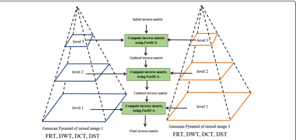
A flow diagram of the proposed method is depicted in Fig.6, which is also described by the following steps:

Step 1: Decompose the mixed image into different transforms using the finite ridgelet transform (FRT), wavelet transform (WT), discrete sine transform (DST), and discrete cosine transform (DCT).

Step 2: Apply a pyramid construction on each transform to obtain the different scale components of each transform in each pyramid level. We chose three levels of pyramid construction in the present work, while it can be extended to a larger number of levels.

Step 3: Conduct a separation operation on all the pyramid levels in each transform and calculate the inverse matrix (un-mixing matrix). The operation proceeds from level 3 (the smallest scale) towards level 1 (the largest scale). In level 3 of pyramid component, we start with a random matrix to calculate the values of inverse matrix. The output values of estimating inverse matrix from level 3 are used as the input matrix to update the inverse matrix values for level 2. The updated output of the inverse matrix from level 2 is in turn used as the input matrix for level 1 to calculate the final values of the inverse matrix. The final estimated values of the inverse matrix are applied to the original mixed image to extract accurate separated images in step 4.

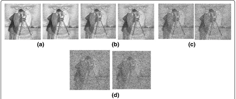
Step 4: Calculate an estimate of the separated image using the mixed image with the calculated inverse matrix. Fig. 9Mixing results at several noise level.a4 dB.b−5 dB.c−10 dB.d−15 dB

(9)

Fig. 10Estimated results of separated image at noise level 4 dB.aProposed method (FRT with pyramid).bFRT without pyramid.cDWT with pyramid.dTime with pyramid.eDWT without pyramid.fTime without pyramid.gDCT with pyramid.hDST with pyramid.iDCT without pyramid.jDST without pyramid

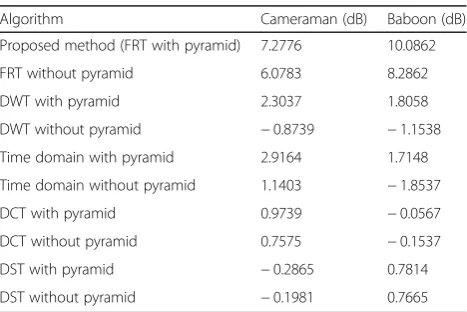
Table 1SNR of overall separation performances on image mixtures

Algorithm Cameraman (dB) Baboon (dB)

Proposed method (FRT with pyramid) 7.2776 10.0862

FRT without pyramid 6.0783 8.2862

DWT with pyramid 2.3037 1.8058

DWT without pyramid −0.8739 −1.1538

Time domain with pyramid 2.9164 1.7148

Time domain without pyramid 1.1403 −1.8537

DCT with pyramid 0.9739 −0.0567

DCT without pyramid 0.7575 −0.1537

DST with pyramid −0.2865 0.7814

DST without pyramid −0.1981 0.7665

Table 2PSNR of overall separation performances on image mixtures

DWT without pyramid 7.9213 4.5781

Time domain without pyramid 7.5340 7.1717

DCT with pyramid 6.5915 5.1941

DCT without pyramid 6.3751 4.77

DST with pyramid 5.3311 6.1143

(10)

ICA has been regarded as one of the most efficient ap-proaches reported in different fields. It provides advantages of fast convergence and straightforward implementation. Figure 7 illustrates a flowchart that realizes the fast inde-pendent component analysis (FastICA) approach [32]:

Next, we introduce several performance metrics to evaluate the image separation results for each given method, which are also described in [33–35].

(i) Signal-to-noise ratio (SNR):

SNR¼10 log10

PM−1 x¼0

PN−1 y¼0f

2

x;y ð Þ

PM−1 x¼0

PN−1

y¼0 f xð ;yÞ−~f xð ;yÞ

2 0 B @ 1 C

AdB ð20Þ

Here, the size of the image isN×M, while f(x,y) rep-resents the original image and ~fðx;yÞ an estimated image.

(ii) Root mean square error (RMSE):

RMSE¼

ffiffiffiffiffiffiffiffiffiffiffiffiffiffiffiffiffiffiffiffiffiffiffiffiffiffiffiffiffiffiffiffiffiffiffiffiffiffiffiffiffiffiffiffiffiffiffiffiffiffiffiffiffiffiffiffiffiffiffiffiffiffiffiffiffiffiffiffiffiffiffiffiffi

1

MN

X_M−1 x¼0

X_N−1

y¼0 f xð ;yÞ−~f xð ;yÞ

2

r

ð21Þ

RMSE is to measure the square error between two im-ages. It considers image degradation as perceived vari-ation in informvari-ation.

(iii) Peak signal-to-noise ratio (PSNR):

PSNR¼20 log₁₀ 1 RMSE

dB ð22Þ

PSNR is one of the most widely used metrics for evaluating the quality of estimated image. The higher the PSNR values are, the higher quality the estimation output provides.

(iv) Normalized cross-correlation (NCC):

NCC¼

PM−1 x¼0

PN−1

y¼0 f xð ;yÞ~f xð ;yÞ

h

P_M−1

x¼0 P_N−1

y¼0ðf xð ;yÞÞ2

ð23Þ

NCC is another common performance metric that is useful to compare the estimation results from different source images.

5 Experiment result and discussion

A computer simulation is presented in this section to evaluate the performance of the proposed approach after the image was mixed. In all experiments, test images were used which were extracted from a standard image database. We assumed that the mixed images are cor-rupted by an additive white Gaussian noise (AWGN) with zero mean and unit variance to illustrate the visual aspect of the various mixed images; we reported in Fig.9 one of each noisy mixture in several noise levels.

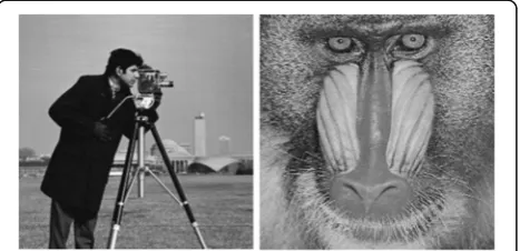
We have conducted experiments on the images of Fig.8and obtained better image separation results from the proposed separation method compared with other separation methods. Due to the space restriction of the paper, we summarize the detailed experiment results with Cameraman and Baboon images. Figure 10 shows the experimental results with Cameraman and Baboon images using the proposed separation method and vari-ous other methods.

These test images are created by a convolutional mixing process using a set of mixing matrices gener-ated randomly by MATLAB, and the criteria of this matrix are normally distributed random numbers.

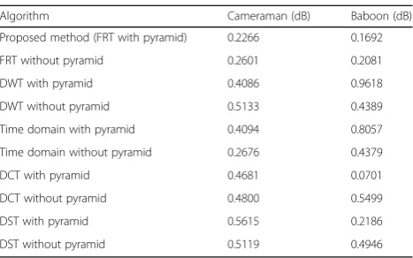
Table 3RMSE of overall separation performances on image mixtures

DWT without pyramid 0.5133 0.4389

Time domain without pyramid 0.2676 0.4379

DCT with pyramid 0.4681 0.0701

DCT without pyramid 0.4800 0.5499

DST with pyramid 0.5615 0.2186

DST without pyramid 0.5119 0.4946

Table 4NCC of overall separation performances on image mixtures

DWT without pyramid −0.2206 −0.1886

Time domain without pyramid 0.2192 −0.4878

DCT with pyramid 0.1109 −0.0611

DCT without pyramid −0.0842 0.0141

DST with pyramid −0.0896 1.1536

DST without pyramid 0.0264 0.0848

(11)

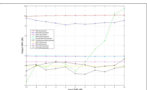
Fig. 11Output SNR vs. input SNR for Cameraman image overall separation performances

(12)

Fig. 13Output PSNR vs. input SNR for Cameraman image overall separation performances

Fig. 14Output PSNR vs. input SNR for Baboon image overall separation performances

(13)

Fig. 15Output RMSE vs. input SNR for Cameraman image overall separation performances

(14)

Fig. 17Output NCC vs. input SNR for Cameraman image overall separation performances

Fig. 18Output NCC vs. input SNR for Baboon image overall separation performances

(15)

Also, Fig. 9 shows the result of mixing process at dif-ferent noise level.

As a result of the experiments, the separated images are shown in Fig. 10. The numerical results of these experiments are included in Tables 1, 2, 3, and 4 at noise level 4 dB. These tables give an image quality comparison between separation algorithms, revealing the superiority of the proposed algorithm at noise level 4 dB. We used SNR, PSNR, RMSE, and NCC to evaluate the estimation quality of separated images.

As illustrated by Fig.10and from Tables1,2,3, and4, the proposed approach performs preliminary separation better than the conventional separation methods based on the time domain, wavelet transform, and trigonomet-ric transform. We can observe that the resulting images of Fig. 10a separated by the proposed RT with homo-morphic method has better quality than other images of Fig.10b–j separated by various different methods.

From Tables1,2,3, and4, it can be observed that the proposed RT with pyramid operation produces higher quality and efficiency compared with all other ap-proaches tested in our experiments. Tables 1 and 2 prove that the SNR and PSNR of the images separated by the proposed method are higher than those of all the other methods. Table 3 indicates that the RMSE of the resulting images separated by the pyramid operation with FRT is the best compared with all other methods considered in our experiments. In addition, as illustrated in Table 4, the NCC of the proposed technique shows a value closer to 1 than any other methods do. Here, an NCC result of 1 is the best possible result. From the ex-perimental results of Tables1,2, 3, and4, it is observed that the separation quality of the time domain-based method is relatively low. This result follows from the fact that the sources must satisfy statistical independ-ence to allow FastICA methods to achieve high-quality separation results.

Figures 11, 12, 13, 14, 15, 16, 17, and 18 plot an extensive set of simulation results measured with a wide range of noise levels. These results compare the separation quality of the tested images using various evaluation metrics including SNR, PSNR, RMSE, and NCC. Figures 11 and 12 present the SNR output of the separated images for Cameraman and Baboon, re-spectively. These figures demonstrate the performance comparison of the proposed BSS method with respect to the other methods at different input noise levels. It shows that the proposed method provides the highest performance. For example, the proposed FRT with pyramid method achieves an SNR of higher than 7 dB for the Baboon image, whereas the DCT with-out pyramid method gives an SNR as low as 0.5 dB. Figures 13 and 14 illustrate the PSNR measurement of the separated images, where the proposed method

can obtain PSNR values of 15 dB or higher, whereas other methods provide much poorer PSNR values in the range of 4~14 dB.

On the other hand, Figs. 15 and 16 demonstrate the output of RMSE. In the RMSE results, the lowest curve indicates the best result. We can observe that the pro-posed method produces an RMSE value of 0.25 or lower, which is 0.2~0.6 lower than other methods. Figures 17 and 18illustrate the simulation results of NCC. It is ob-served that the proposed method produces an NCC value very close to 1, while other methods provide much NCC values in the range of−0.1~ 4.

6 Conclusions

This paper addressed the blind image separation problem by introducing a new image separation technique based on a novel concept of pyramid pro-cessing and ridgelet transform. The proposed ap-proach first uses FRT domain coefficients to obtain the frequency components. It then applies a pyramid processing to estimate the mixing matrix by con-structing the different level scales to extract more details in information and remove redundant infor-mation. We conducted an extended set of simulation experiments using various image separation methods that employ the proposed FRT as well as other methods including DWT, time domain, DCT, and DST along with pyramid and non-pyramid opera-tions, respectively. The experimental results demon-strate that the proposed method outperforms all other methods that we tested. In summary, it pre-sents PSNR values of 12~16 dB under a wide range of noise condition, while all other methods provide much poor PSNR values of 4~10 dB under the same noise condition. The proposed method, therefore, appears to be an efficient approach to separate mixed images even under noisy conditions.

Abbreviations

BSS:Blind source separation; DCT: Discrete cosine transform; DST: Discrete sine transform; DWT: Discrete wavelet transform;

EEG: Electroencephalography; FastICA: Fast independent component analysis; fMRI: Functional magnetic resonance imaging; FRAT: Finite Radon Transform; FRT: Finite ridgelet transform; ICA: Independent component analysis; ITW: Idiopathic toe walking; NCC: Normalized cross-correlation; PR: Perfect reconstruction; PSNR: Peak signal-to-noise ratio; RAT: Radon Transform; RMSE: Root mean square error; RT: Ridgelet transform; SNR: Signal-to-noise ratio; WT: Wavelet transform

Funding

(16)

Authors’contributions

MYA and HWK designed the proposed algorithm together. MYA implemented it with MATLAB. Both authors wrote and approved the final manuscript. The corresponding author is HWK ([email protected]).

Competing interests

The authors declare that they have no competing interests.

Publisher’s Note

Springer Nature remains neutral with regard to jurisdictional claims in published maps and institutional affiliations.

Author details

1

Department of Electronic Engineering, College of Electrical and Computer Engineering, Chungbuk National University, Cheongju City, South Korea.

2_{Engineering Department, Nuclear Research Center, Atomic Energy Authority,}

Cairo City, Egypt.

Received: 12 December 2017 Accepted: 14 May 2018

References

1. A Cichocki, S Amari,Adaptive blind signal and image processing: learning algorithms and applications(Wiley, New York, 2005)

2. YW Wei, Y Wangb, Dynamic blind source separation based on source-direction prediction. Neurocomputing185, 73–81 (2016)

3. S Ali, NA Khan, M Haneef, et al., Blind source separation schemes for mono-sensor and multi-mono-sensor systems with application to signal detection. Circuits Systems Signal Process36(11), 4615–4636 (2017)

4. LT Duarte, JMT Romano, C Jutten, KY Chumbimuni-Torres, LT Kubota, Application of blind source separation methods to ion-selective electrode arrays in flow-injection analysis. IEEE Sensors J14(Issue 7), 2228_–2229 (2014) 5. XL Li, Adali, Independent component analysis by entropy bound

minimization. IEEE Trans. Signal Process.58(10), 5151–5164 (2010) 6. T Adali, VD Calhoun, Complex ICA of brain imaging data. IEEE Signal

Process. Mag.24(5), 136_–139 (2007)

7. R Chai, GR Naik, TN Nguyen, SH Ling, Y Tran, A Craig, HT Nguyen, Driver fatigue classification with independent component by entropy rate bound minimization analysis in an EEG-based system. IEEE J. Biomed. Health Inform.21(3), 715_–24 (2016)

8. G Pendharkar, GR Naik, HT Nguyen, Using blind source separation on accelerometry data to analyze and distinguish the toe walking gait from normal gait in ITW children. Biomed. Signal Process. Contr.13, 41–49 (2014) 9. A Hyvärinen, Survey on independent component analysis. Neural

Computing Surveys2, 94–128 (1999)

10. A Hyvärinen, E Oja, Independent component analysis: algorithms and applications. Neural Netw.13(4–5), 411–430 (2000)

11. JF Cardoso, B Laheld, Equivariant adaptive source separation. IEEE Transaction Signal Process.44, 3017–3030 (1996)

12. E Oja, A Hyvärinen, J Karhunen,Independent component analysis(Wiley, United States of America, 2001)

13. X He, F He, A He, Super-Gaussian BSS using fast-ICA with Chebyshev-Pade approximant. Circuits Systems Signal Process37(1), 305–341 (2018) 14. MSC Almeida, LB Almeida, Wavelet-based separation of nonlinear

show-through and bleed-show-through image mixtures. Neurocomputing72(1–3), 57– 70 (2008)

15. MT Ozgen, EE Kuruoglu, D Herranz, Astrophysical image separation by blind time-frequency source separation methods. Digit Signal Process, 360–369 (2009, 2009)

16. X J-d Chuan, H Dan, X Hai-hua, A new blind image source separation algorithm based on feedback sparse component analysis. Signal Process.93, 288–296 (2013)

17. S Belaid, J Hattay, W Naanaa, et al. A new multi-scale framework for convolutive blind source separation. SIViP.10, 1203 (2016) 18. S Kim, CD Yoo, Underdetermined blind source separation based on

subspace representation. IEEE Trans. Signal Process.,57(7), 2604–14 (2009) 19. N Besic, G Vasile, J Chanussot, S Stankovic, Polarimetric incoherent target decomposition by means of independent component analysis. IEEE Trans. Geosci. Remote Sens.53(3), 1236–1247 (2015)

20. C Hu, Z Xu, Y Liu, L Mei, L Chen, X Luo, Semantic link network based model for organizing multimedia big data. IEEE Trans Emerg Top Comput.,2(3), 376–87 (2014)

21. XC Yu, JD Xu, D Hu, Xing HH, A new blind image source separation algorithm based on feedback sparse component analysis. Signal Process.,

93(1), 288_–96 (2013)

22. Y Zhang, D Yang, R Qi, Z Gong, Blind image separation based on reorganization of block DCT. Multimedia Tools and Applications (2016) 23. Burt and Adelson,“The Laplacian pyramid as a compact image code,”IEEE

Transactions on Communications, Vol. COM-31, no. 4, pp. 532_–540, 1983. 24. L Xiaoa, C Lia, Z Wub, T Wangc, An enhancement method for X-ray image

via fuzzy noise removal and homomorphic filtering. Neurocomputing195, 56–64 (2016)

25. E.J. Candes, Ridgelets:_“theory and applications_”, Ph.D. thesis, Department of Statistics, Stanford University, 1998.

26. E.J. Candes, D.L. Donoho,“Curvelets, Tech. report”, Department of Statistics, Stanford University, 1999.

27. E.J. Candes, D.L. Donoho,_“Curvelets: a surprisingly effective nonadaptive representation for objects with edges”, Tech. report, Department of Statistics, Stanford University, 2000.

28. J-L Starck, EJ Candès, DL Donoho, The curvelet transform for image denoising. IEEE Trans. Image Process.,11(6), 670_–84 (2002) 29. Q Huang, B Hao, S Chang, Adaptive digital ridgelet transform and its

application in image denoising. Digital Signal Processing52, 45–54 (2016) 30. EJ Candes, DL Donoho, Ridgelets: a key to higher dimensional

intermittency? Philos. Trans. R. Soc. Lond.A357, 2459_–2509 (1999) 31. JS Walker,A primer on wavelets and their scientific applications(CRC Press,

Boca Raton, 1999)

32. KR Rao, P Yip,Discrete cosine transform(Academic, New York, 1990) 33. A Hyvärinen, E Oja, A fast fixed-point algorithm for independent

component analysis. Neural Comput.9(7), 1483–1492 (1997) 34. H Hammam, AA Elazm, ME Elhalawany, et al., Blind separation of audio

signals using trigonometric transforms and wavelet denoising. Int J Speech Technol,13, 1 (2010)

35. Z Wang, AC Bovik, HR Sheikh, EP Simoncelli, Image quality assessment: from error visibility to structural similarity. IEEE Trans. Image Process.13(4), 600– 612 (2004)