Durham Research Online
Deposited in DRO:08 October 2019
Version of attached le: Accepted Version
Peer-review status of attached le: Peer-reviewed
Citation for published item:
Perrakis, Konstantinos and Ntzoufras, Ioannis and Tsionas, Efthymios G. (2014) 'On the use of marginal posteriors in marginal likelihood estimation via importance sampling.', Computational statistics data analysis., 77 . pp. 54-69.
Further information on publisher's website: https://doi.org/10.1016/j.csda.2014.03.004
Publisher's copyright statement:
c
2014 This manuscript version is made available under the CC-BY-NC-ND 4.0 license http://creativecommons.org/licenses/by-nc-nd/4.0/
Additional information:
Use policy
The full-text may be used and/or reproduced, and given to third parties in any format or medium, without prior permission or charge, for personal research or study, educational, or not-for-prot purposes provided that:
• a full bibliographic reference is made to the original source
• alinkis made to the metadata record in DRO
• the full-text is not changed in any way
The full-text must not be sold in any format or medium without the formal permission of the copyright holders. Please consult thefull DRO policyfor further details.
On the use of marginal posteriors in marginal
likelihood estimation via importance sampling
Konstantinos Perrakis
1, Ioannis Ntzoufras
1and Efthymios G. Tsionas
21Department of Statistics, Athens University of Economics and Business, Greece 2Department of Economics, Athens University of Economics and Business, Greece
Abstract
We investigate the efficiency of a marginal likelihood estimator where the product of the marginal posterior distributions is used as an importance sam-pling function. The approach is generally applicable to multi-block parameter vector settings, does not require additional Markov Chain Monte Carlo (MCMC) sampling and is not dependent on the type of MCMC scheme used to sample from the posterior. The proposed approach is applied to normal regression models, finite normal mixtures and longitudinal Poisson models, and leads to accurate marginal likelihood estimates.
Keywords: Finite normal mixtures, importance sampling, marginal posterior, marginal likelihood estimation, random effect models, Rao-Blackwellization
1
Introduction
The problem of estimating the marginal likelihood has received considerable attention during the last two decades. The topic is of importance in Bayesian statistics as it is associated with the evaluation of competing hypotheses or models via Bayes factors and posterior model odds. Consider, briefly, two competing models M1 and M2 with
corresponding prior probabilities π(M1) and π(M2) = 1−π(M1). After observing a
data vector y, the evidence in favour of M1 (or against M2) is evaluated through the
odds of the posterior model probabilities p(M1|y) and p(M2|y), that is,
p(M1|y) p(M2|y) = m(y|M1) m(y|M2) × π(M1) π(M2) .
The quantityB12=m(y|M1)/m(y|M2) is the ratio of the marginal likelihoods or prior
predictive distributions ofM1 and M2 and is called the Bayes factor ofM1 versus M2.
The Bayes factor can also be interpreted as the ratio of the posterior odds to the prior odds. WhenM1 and M2 are assumed to be equally probable a-priori, the Bayes factor
The marginal likelihood of a given model Mk associated with a parameter
vec-tor θk is essentially the normalizing constant of the posterior p(θk|y, Mk), obtained
by integrating the likelihood function l(y|θk, Mk) with respect to the prior density
π(θk|Mk), i.e.
m(y|Mk) = Z
l(y|θk, Mk)π(θk|Mk)dθk. (1)
The integration in (1) may be evaluated analytically for some elementary cases. Most often, it is intractable thus giving rise to the marginal likelihood estimation problem. Numerical integration methods can be used as an approach to the problem, but such techniques are of limited use when sample sizes are moderate to large or when vector
θk is of large dimensionality. In addition, the simplest Monte Carlo (MC) estimate,
which is given by b m(y|Mk) = N−1 N X n=1 l(y|θ(kn), Mk), (2)
using draws {θ(kn) : n = 1,2, ..., N} from the prior distribution is extremely unstable when the posterior is concentrated in relation to the prior. This scenario is frequently met in practice when flat, low-information prior distributions are used to express prior ignorance. A detailed discussion regarding Bayes factors and marginal likelihood estimation is provided by Kass and Raftery (1995).
It is worth noting that the problem of estimating (1) can be bypassed by consid-ering model indicators as unknown parameters. This option has been investigated by several authors (e.g. Green, 1995, Carlin and Chib, 1995, Dellaportas et al., 2002) who introduce MCMC algorithms which sample simultaneously over parameter and model space and deliver directly posterior model probabilities. However, implementation of these methods can get quite complex since they require enumeration of all compet-ing models and specification of tuncompet-ing constants or “pseudopriors” (dependcompet-ing upon approach) in order to ensure successful mixing in model space. Moreover, since these methods focus on the estimation of posterior model probabilities, accurate estimation of the marginal likelihoods and/or Bayes factors will not be feasible in the cases where a dominating model exists in the set of models under consideration; tuning, following the lines of Ntzoufras et al. (2005), might be possible but is typically inefficient and time consuming.
In contrast, “direct” methods provide marginal likelihood estimates by utilizing the posterior samples of separate models. These methods are usually simpler to implement and are preferable in practice when the number of models under consideration is not large, namely when it is practically feasible to obtain a posterior sample for each of the competing models. Work along these lines includes the Laplace-Metropolis method (Lewis and Raftery, 1997), the harmonic-mean and the prior/posterior mixture im-portance sampling estimators (Newton and Raftery, 1994), bridge-sampling methods (Meng and Wong, 1994), candidate’s estimators for Gibbs sampling (Chib, 1995) and Metropolis-Hastings sampling (Chib and Jeliazkov, 2001), annealed importance sam-pling (Neal, 2001), importance-weighted marginal density estimators (Chen, 2005)
and nested sampling approaches (Skilling, 2006). More recently, Raftery et al. (2007) presented a stabilized version of the harmonic-mean estimator, while Friel and Pettitt (2008) and Weinberger (2012) proposed new approaches based on power posteriors and Lebesgue integration theory, respectively. It is worth mentioning that Bayesian evidence evaluation is also of particular interest in the astronomy literature where nested sampling is commonly used for marginal likelihood estimation (e.g. Feroz et al., 2009; Feroz et al., 2011). Recent reviews comparing popular methods based on MCMC sampling can be found in Friel and Wyse (2012) as well as in Ardia et al. (2012). Alternative approaches for marginal likelihood estimation include sequential Monte Carlo (Del Moral et al., 2006) and variational Bayes (Parise and Welling, 2007) methods.
In this paper we propose using the marginal posterior distributions on importance sampling estimators of the marginal likelihood. The proposed approach is particularly suited for the Gibbs sampler, but it is also feasible to use for other types of MCMC algorithms. The estimator can be implemented in a straightforward manner and it can be extended to multi-block parameter settings without requiring additional MCMC sampling apart from the one used to obtain the posterior sample.
The remainder of the paper is organized as follows. The proposed estimator and its variants are discussed in Section 2. In Section 3 the method is applied to nor-mal regression models, to finite nornor-mal mixtures and also to hierarchical longitudinal Poisson models. Concluding remarks are provided in Section 4.
2
The proposed estimator
In the following we first introduce the proposed estimator in a two block setting. The more general multi-block case is considered next, explaining why the estimator will be useful in such cases. We further present details concerning the implementation of the proposed approach when the model formulation includes latent variables or nuisance parameters that are not of prime interest for model inference. The section continues with a description of the different estimation approaches of the posterior marginal distributions used as importance functions. We conclude with a note on a convenient implementation of the estimator for models where the posterior distribution becomes invariant under competing diffuse priors and brief remarks about the calculation of numerical standard errors. In the remaining of the paper, the dependence to the model indicator Mk (introduced in the previous section) is eliminated for notational
simplicity.
2.1
Introducing the estimator in a two-block setting
Let us consider initially the 2-block setting wherel(y|θ,φ) is the likelihood of the data conditional on parameter vectors θ = (θ1, θ2, ..., θp)T and φ= (φ1, φ2, ..., φq)T, which
π(θ|φ)π(φ), a-priori. In general, one can improve the estimator in (2) by introducing a proper importance sampling densityg and then calculate the marginal likelihood as an expectation with respect tog instead of the prior, i.e.
m(y) = Z l(y|θ,φ)π(θ,φ) g(θ,φ) g(θ,φ)d(θ,φ) = Eg l(y|θ,φ)π(θ,φ) g(θ,φ) .
This quantity can be easily estimated as
b m(y) = N−1 N X n=1 l(y|θ(n),φ(n))π(θ(n),φ(n)) g(θ(n),φ(n)) ,
where θ(n) and φ(n), for n = 1,2, ..., N, are draws from g. Theoretically, an ideal importance sampling density is proportional to the posterior. In practice, we seek densities which are similar to the posterior and easy to sample from.
Given this consideration, we propose to use the product of the marginal posterior distributions as importance sampling density, i.e. g(θ,φ)≡p(θ|y)p(φ|y). Under this approach
m(y) =
Z Z l(y|θ,φ)π(θ,φ)
p(θ|y)p(φ|y) p(θ|y)p(φ|y)dθdφ, which yields the estimator
b m(y) = N−1 N X n=1 l(y|θ(n),φ(n))π(θ(n),φ(n)) p(θ(n)|y)p(φ(n)|y) . (3) Note that the only twist in (3) is that the draws θ(n) and φ(n), for n= 1,2, ..., N, are draws from the marginal posteriors p(θ|y) and p(φ|y) and not from the joint poste-rior p(θ,φ|y). In most cases the marginal posterior distributions will not be known, nevertheless, this does not constitute a major obstacle neither for sampling from the marginal posteriors nor for calculating the marginal probabilities which appear in the denominator of (3); the former issue is discussed here, the latter is handled in Section 2.4.
It is straightforward to see that the product marginal posterior is the optimal im-portance sampling density when θ and φ are independent a-posteriori, since in this case p(θ|y)p(φ|y) =p(θ,φ|y) leading to the zero-variance estimator. Although pos-terior independence is not frequently met in practice, the product marginal pospos-terior can serve as a good approximation to the joint posterior even if θ and φ are not completely independent a-posteriori. First, it has exactly the same support as the joint posterior. Second, the blocking of the parameters can be such that the param-eter blocks are close to orthogonal regardless whether the elements within θ and φ
are strongly correlated. Furthermore, appropriate reparameterizations can be used in order to form parameter blocks which are orthogonal or close to orthogonal (see e.g. Gilks and Roberts, 1996). Moreover, in generalized linear models the augmentation scheme of Ghosh and Clyde (2011) can be used to obtain orthogonal parameters.
It is worth noting that the estimator in (3) is similar to the Markov chain impor-tance sampling approach described in Botev et al. (2012) and the marginal likelihood estimator proposed in Chan and Eisenstat (2013) based on the cross-entropy method. Botev et al. (2012) show that the product of the marginals is the best importance sam-pling density – in the sense of minimizing the Kullback-Leibler divergence with respect to the zero-variance importance sampling density – among all product form impor-tance sampling densities, given that the zero-variance density is also decomposable in product form. Similarly, Chan and Eisenstat (2013) locate the importance sampling density minimizing Kullback-Leibler divergence with respect to block-independent fac-torizations of the joint posterior from distributions belonging to the same parametric families as the priors. The approach presented here differentiates from the above esti-mators since we consider directly the marginal posteriors and “manipulate” the joint MCMC sample in order to construct marginal samples, thus avoiding further impor-tance sampling and leaving estimation of marginal densities as the main issue to deal with.
In general, marginal posterior samples can be obtained from any MCMC algorithm. The only problem is that a single MCMC chain corresponds to a sample from the joint distribution, with non-zero covariance between parameter blocks. One option is to use a different MCMC run for each block of parameters. In this case, one can calculate the estimator in (3) by using draws θ(n), φ(n) coming from two independent MCMC samples of equal size N. Nevertheless, this approach can considerably increase the number of MCMC iterations, especially for a large number of parameter blocks. In addition, the approach is not economical in the sense that onlyN posterior draws are used from a total sample of 2N draws.
A simple and more efficient solution is to re-order a single MCMC chain in such a way that it does not correspond to a sample from the joint posterior distribution. This can be easily implemented by systematically permuting either the sampled values of
θ or those of φ. For instance, consider one MCMC chain where the initial MCMC draws are indexed as {θ(n),φ(n) : n = 1,2, ..., N1, N1 + 1, N1 + 2, ..., N} where N1 =
N/2. Then, one can simply re-order the sample of φ as {φ(n1) : n
1 = N1 + 1, N1 +
2, ..., N,1,2, , ..., N1}and join the set of draws {θ(n),φ(n1)}, thus forming a sample of
paired realizations from the distribution g(θ,φ) = p(θ|y)p(φ|y). Obviously, when the paired sample has been formed, the distinction between the two sets of indices becomes irrelevant and a common index may be adopted as presented in equation (3). Reordering is trivial in implementation regardless of the number of parameter blocks; the only initial requirement is that the size of the final MCMC sampleN must be dividable with the number of blocks, say B, so that B independent reorderings of the MCMC chain can be formed. This line of reasoning also holds for cases of multiple-chain MCMC sampling, which is a frequent MCMC strategy favoured mainly on the basis of MCMC convergence checks (e.g. Gelman and Rubin, 1992). For such cases, one can re-order the within-chain posterior samples in a similar manner to that previously described, and then form a joined sample from the multiple re-ordered chains.
Another, even simpler, alternative for removing correlations between marginal sam-ples is to randomly permute each sample. Results using this approach will be similar to the above systematic re-ordering, except in extreme, unlikely cases where randomly permuted samples with non-zero sample correlation are generated by chance. Irrespec-tive of the reorderding scheme used, for the remainder of this paper we use a common index n across parameter blocks, referring to joined independent block samples.
2.2
Extension to multi-block settings
Generalization to multi-block hierarchical settings is straightforward. Consider B
blocks θ1,θ2, ...,θB; in this case the product of the B marginal posteriors is used as
importance sampling density and
m(y) = Z ... Z l(y|θ 1, ...,θB)π(θ1, ...,θB) B Q i=1 p(θi|y) B Y i=1 p(θi|y)dθi,
which yields the following estimator
b m(y) =N−1 N X n=1 l(y|θ(1n), ...,θ(Bn))π(θ(1n), ...,θ(Bn)) B Q i=1 p(θ(in)|y) . (4)
Note that the estimator in (4) may also refer to multiple unidimensional blocks where each parameter forms one block. The advantage of such an estimator raises from the fact that it is easy to construct good approximations of univariate marginal posterior distributions. On the other hand, any possible gain in the efficiency earned from the construction of good approximating densities for the marginal posteriors might be moderated by the use of an importance function which assumes overall independency. Therefore, the most efficient strategy is to choose blocks of minimal size constituted only by highly correlated parameters, which have at the same time weak between-block corrrelations. Of course, quite often the model design is such that this condition is already met, e.g. for reasons of efficient MCMC mixing. In addition, for cases of Gibbs sampling the natural blocking is the most convenient to use, since in such cases marginal posterior densities can be estimated accurately even for high-dimensional parameter blocks (see Section 2.4 for more details).
2.3
Handling latent variables and nuisance parameters
Many hierarchical models include a block componentu, usually not of main inferential interest, which is associated with a hyperparameter vectorωthrough the relationship
π(u,ω) = π(u|ω)π(ω). For instance, u may be a random effect vector or a latent vector used to facilitate posterior simulation through Gibbs sampling as in the data
augmentation setting introduced in Tanner and Wong (1987). In such cases infer-ence usually focuses on the marginal sampling likelihood by integrating out u. For example, when there is only one parameter blockθ, the marginal sampling likelihood is l(y|θ,ω) = R
l(y|θ,u)π(u|ω)du. In this case, a marginal likelihood estimate is obtained through equation (3), where φ is simply replaced by ω. The extension to the multi-block setting is essentially the same as in (4), only with the addition of ω, specifically b m(y) =N−1 N X n=1 l(y|θ(1n), ...,θ(Bn),ω(n))π(θ(1n), ...,θB(n))π(ω(n)) B Q i=1 p(θ(in)|y)p(ω(n)|y) . (5)
Alternatively, there is also the option of working with the hierarchical likelihood and including u in the estimation process, i.e.
b m(y) =N−1 N X n=1 l(y|θ(1n), ...,θB(n),u(n))π(θ(n) 1 , ...,θ (n) B )π(u(n)|ω(n))π(ω(n)) B Q i=1 p(θ(in)|y)p(u(n)|y)p(ω(n)|y) . (6)
The latter approach is less practical to implement as it requires evaluation of p(u|y). In addition, marginalization over u will in general lead to more precise marginal likelihood estimates due to scaling down the parameter space; see Vitoratou et al.
(2013) for further details. Therefore, estimator (5) is overall preferable to estimator (6), except perhaps in cases where the likelihood in (5) is not available analytically and also estimation of p(u|y) is easy to handle based on the methods discussed next.
2.4
Estimating marginal posterior densities
As seen so far, the proposed approach is fairly simple to implement. The only re-maining issue is the evaluation of the marginal posterior probabilities appearing in the denominators of estimators (3)–(6). Here we discuss some different approaches that can be adopted.
A first simple approach is to assume normality either directly or indirectly. Let us consider, for instance, the 2-block setting of Section 2.1 with parameter blocks
θ and φ. Suppose, for instance, that θ relates to a vector of means or a vector of regression parameters. Then, for moderate to large sample sizes, a reasonable option is to assume thatθ|y∼N(θ,Σθ), where θ and Σθ are the estimated posterior mean
vector and variance-covariance matrix from the MCMC output, respectively. Vector
φ, on the hand, may refer to a vector of disperion parameters, where the assumption of normality may not be suitable. One stategy, often sufficient in many cases, is to assume that a transformationx=t(φ) is approximately normal, i.e. x|y∼N(x,Σx),
and consequentlyp(φ|y) = p(x|y)|dt−1dx(x)|−1 for an appropriate invertible functiont(·).
An alternative is to mimic the marginal posteriors by adopting appropriate dis-tributional assumptions and matching parameters to posterior moments. This option
is more suitable when the assumption of normality is not particularly supported and appropriate transformation functions are hard to find. In such cases, one can also consider a wide range of options based on multivariate kernel methods (e.g. Scott, 1992) as an efficient alternative.
Moreover, when implementing Gibbs sampling where the normalizing constants of the full conditional distributions are known, marginal posterior densities can be esti-mated through an efficient, simulation-consistent technique referred as Rao–Blackwellization by Gelfand and Smith (1990). Consider, for instance, the B parameter block setting of Section 2.2; the Rao-Blackwell estimates in this case are
b p(θ1|y) = L−1 L X l=1 p(θ1|θ(2l), . . . ,θ (l) B,y), b p(θb|y) = L−1 L X l=1 p(θb|θ (l) 1 , . . . ,θ (l) b−1,θ (l) b+1, . . . ,θ (l) B,y) for b= 2, . . . , B−1 b p(θB|y) = L−1 L X l=1 p(θB|θ (l) 1 , . . . ,θ (l) B−1,y).
Note that not all N posterior draws need to be used; usually a sufficiently large subsample of L posterior draws is adequate. For instance, in the examples presented next we find that samples between 200 to 500 draws are sufficient, which significantly reduces computational expense. It should also be noted that Rao-Blackwell estimates must be based on draws from the joint posterior distribution, that is draws from the initial non-permuted MCMC sample.
Finally, for cases of hybrid Gibbs sampling where only some full conditionals are known, one can use a combination of the methods discussed here. Rao-Blackwellization may be used for parameter blocks with known full conditional distributions, whereas for the remaining blocks one can choose among distributional approximations based on moment-fitting and kernel methods.
Estimators (3)–(6) will not be unbiased when approximating the marginal posterior densities using moment-matching strategies. Nevertheless, in practice such “proxies” can be very accurate for univariate as well as multivariate distributions. For instance, as illustrated in Section 3.3, high-dimensional marginal posteriors are approximated efficiently through multivariate normal distributions. In addition, the degree of bias can be empirically checked by comparing such estimates to the corresponding ones using importance samples from the moment-matched approximating distributions. The latter procedure yields an unbiased estimator of the marginal likelihood and, therefore, small observed differences will imply that the bias introduced is negligible.
2.5
Marginal likelihood estimation for diffuse priors
As known, the marginal likelihood is very sensitive to changes in the prior distribution, whereas the posterior distribution (after a point) is insensitive to the prior as the latter
becomes more and more diffuse. Therefore, a usual drawback of marginal likelihood estimators that are based solely on draws from the posterior distribution is that they are typically not reliable for evaluating the marginal likelihoods of different models when considering diffuse priors (see e.g. Friel and Wyse, 2012).
Nevertheless, this is not the case for the proposed estimator as it incorporates the prior in the estimation of the marginal likelihood. In fact, we can easily adopt estimator (3) in order to estimate the marginal likelihood under different diffuse priors (that have no essential effect on the posterior distribution) using a sample from a single MCMC run. To illustrate this, consider the 2-block setting of Section 2.1 and two diffuse priors π0, π1 under which the posterior distribution remains unchanged,
i.e. p0 ≡ p1. Let us assume that draws {θ(n),φ(n) : n = 1,2, ..., N} are available
from an initial MCMC run and that the marginal likelihoodm0 under π0 has already
been estimated through (3). Then, the marginal likelihood underπ1 can be accurately
estimated by b m1(y) = N−1 N X n=1 l(y|θ(n),φ(n))π1(θ(n),φ(n)) p0(θ(n)|y)p0(φ(n)|y) . (7)
The estimator in (7) does not require additional MCMC sampling, likelihood evalua-tions or evaluaevalua-tions of the marginal posterior densities since the posterior distribuevalua-tions
p1 and p0 are the same under π1 and π0, respectively; the only extra effort involved is
calculation of the prior probabilitiesπ1(θ(n),φ(n)), for n= 1,2, ..., N.
2.6
Calculating the numerical standard error
The method of batch means provides a straightforward way for calculating the numer-ical or MC error of the estimator. Consider for instance the 2-block setting of Section 2.1; in this case the block-independent posterior sample ζ(n) ≡(θ(n),φ(n)) is divided into K batches ζ(nk)
1 ,ζ (nk)
2 , ...,ζ (nk)
K of size NK, i.e. nk = 1,2, ..., NK and N = KNK,
and one calculates
b mk(y) =NK−1 NK X nk=1 l(y|θ(nk) k ,φ (nk) k )π(θ (nk) k ,φ (nk) k ) p(θ(nk) k |y)p(φ (nk) k |y) , (8)
for k= 1,2, ..., K. Then, an estimate of the standard error is given by
c s.e.(mb(y)) = v u u t 1 K(K−1) K X k=1 [mbk(y)−m(y)] 2 , (9) where m(y) = K−1PK
k=1mbk(y) is the average batch mean estimate. Note that K
must be large enough to ensure proper estimation of the variance (the usual choice is 30 ≤ K ≤ 50) and NK must also be sufficiently large so that the mbk’s are roughly
Alternatively, we can consider the variance estimators of Newey and West (1987) and Geyer (1992) for dependent MCMC draws. Such estimators are suited when systematic re-ordering is used to form the block-independent posterior sample, since, in this case, the posterior dependency patterns will be the same as those of the initial MCMC sample. This is due to the fact that the number of parameter blocks B will be usually much smaller than the size of the posterior sample (B N). Therefore, serial auto-correlations for lags greater than N/B are expected to be negligible (for converged MCMC runs), while auto-correlations of lower order are not affected by the re-ordering.
Finally, checking whether the variance is finite or not can be investigated empiri-cally; if the variance is finite then one should expect that increasing the MCMC sample by a factor of d should lead to a decrease of the standard error estimate by a factor approximately equal to√d. As illustrated in Section 3.4, the variance of the proposed estimator is finite for the examples presented in Section 3.
3
Examples
In this section we apply our method to three common classes of models. First, we con-sider normal linear regression where the true marginal likelihood can be calculated an-alytically, and compare the proposed estimator to other estimators commonly used in practice. The second example concerns finite normal mixture models where marginal likelihood estimation has proven particularly problematic due to non-identifiability. In the third example, we apply the proposed methods to an hierarchical longitudinal Poisson model where the integrated sampling likelihood is analytically unavailable and, furthermore, standard Gibbs sampling cannot be implemented. The section closes with an empirical diagnostic for checking the assumption of finite variance by comparing the corresponding errors from samples of size N and 2N.
In all illustrations, we denote the likelihood functions with l(·), prior densities withπ(·) and posterior or full conditional distributions withp(·). Concerning specific distributional notation, the inverse-gamma density defined in terms of shapeαand rate
βis denoted byIG(α, β), the Dirichlet distribution withkconcentration parameters by Dir(α1, α2, ..., αk) and the p-dimensional inverse-Wishart distribution with ν degrees
of freedom and scale matrix Ψby IWp(ν,Ψ).
3.1
Normal regression models
Here we consider the data set presented in Montgomery et al. (2001, p.128) concern-ing 25 direct current (DC) electric charge measurements (volts) and wind velocity measurements (miles/hour). The goal is to infer about the effect of wind velocity on the production of electricity from a water mill. The models under consideration are
i) M0: the null model with the intercept,
iii) M2: intercept+(x2−x2) and
iv) M3: intercept+(x1−x1)+x21,
where x1 is wind velocity and x2 is the logarithm of wind velocity. Let j denote
the model indicator, i.e. j = 0,1,2,3. The likelihood and prior assumptions are the following y|βj, σj2 ∼ N(Xjβj,Iσ 2 j) βj|σj2 ∼ N(0,Vjσ2j) σj2 ∼ IG(10−3,10−3)
where βj and Xj correspond to the regression vector and design matrix of model j,
respectively, andVj =n2(XjTXj)−1 with n= 25. In relation to the context of Section
2 this is a 2-block setting whereβ ≡θand σ2 ≡φ. Under this conjugate prior design the distributions p(βj|σ2
j,y), p(σj2|βj,y), p(βj|y) and p(σj2|y) are all of known form.
We treat the posterior distribution as unknown and implement a Gibbs sampler in R. Specifically, one Gibbs chain is iterated 10,000 times and the first 1000 iterations are discarded as burn-in, resulting in a final posterior sample of 9,000 draws for each model. We calculate two variations of estimator (3), considering: i) the true marginals
p(βj|y) and p(σ2j|y), and ii) Rao-Blackwell estimates of p(βj|y) andp(σj2|y) based on reduced samples of 200 posterior draws. The two variants are denoted bymb(y)mp and
b
m(y)RB, respectively.
For comparison reasons, we also consider the following commonly used marginal likelihood estimators: the Laplace-Metropolis estimator (Lewis and Raftery, 1997), the importance-weighted marginal density estimator of Chen (2005), the candidate’s estimator from Gibbs sampling (Chib, 1995) and the optimal bridge-sampling estima-tor (Meng and Wong, 1996). For the Laplace-Metropolis we require only the MCMC estimated posterior mean vector and posterior covariance matrix. For the second estimator, which requires specification of approximating densities, we use normal dis-tributions for theβj’s and inverse gamma distributions for the σ2
j’s which mimic the
respective component-wise marginal posteriors through moment-fitting. In addition, the points which maximize the unnormalized posterior density of each model are used as posterior ordinates. In order to apply Chib’s estimator in a realistic context (using reduced Gibbs sampling) the posterior ordinates (the points maximazing the unnor-malized posterior) are decomposed according to the univariate densities. The reduced posterior ordinates are calculated via Rao-Blackwellization based on 9,000 draws from further Gibbs updating (additional sampling is not needed for the simple intercept-mopel). Finally, for the optimal bridge-sampling estimator, which is calculated itera-tively, we utilize the same approximating densities as in the implementation of Chen’s estimator and iterate 1000 times using the geometric bridge-sampling estimates, also presented in Meng and Wong (1996), as starting values. The three additional estima-tors are denoted by mb(y)LM, mb(y)Chen, mb(y)Chib and mb(y)obs, respectively.
In order to calculate MC errors the posterior samples are divided into 30 batches of 300 draws. Batch mean estimates, MC errors and the true marginal log-likelihoods
Estimator Model
M0 M1 M2 M3
Laplace-Metropolis logmb(y)LM -35.1381 -12.3676 -0.4044 -0.9044 (0.0092) (0.0124) (0.0092) (0.0112) Importance-weighted logmb(y)Chen -34.8815 -13.1407 -1.5979 -2.2277
(0.0029) (0.0039) (0.0031) (0.0068) Candidate’s logmb(y)Chib -34.8789 -13.1420 -1.5962 -2.2337
(0.0020) (0.0028) (0.0023) (0.0067) Optimal bridge-sampling logmb(y)obs -34.8807 -13.1412 -1.5979 -2.2294
(0.0011) (0.0019) (0.0022) (0.0030) Proposed method
Exact marginals logmb(y)mp -34.8786 -13.1420 -1.5932 -2.2302 (0.0023) (0.0035) (0.0030) (0.0030) Rao-Blackwellization logmb(y)RB -34.8782 -13.1405 -1.5919 -2.2280
(0.0023) (0.0030) (0.0030) (0.0033)
Target value logm(y) -34.8797 -13.1429 -1.5953 -2.2270
Table 1: Estimated marginal log-likelihood values compared with true values for Ex-ample 1; average batch mean estimates (MC errors in parentheses) are presented using 30 batches of size 300.
are presented in Table 1. In practical terms, we found mb(y)LM being the easiest to compute. On the other hand, this estimator performs poorly in comparison to the others, as seen in Table 1. Variations of mb(y)LM based on multivariate medians (L1
centers) and maximum density points of the unnormalized posteriors (not presented here) did not yield substantially different estimates. In contrast, estimatorsmb(y)Chen,
b
m(y)Chib and mb(y)obs perform substantially better. Implementation for mb(y)obs is in general somewhat more complicated in comparison tomb(y)Chen as it requires an itera-tive solution in addition to specification of approximating densities, whereas mb(y)Chib requires additional Gibbs sampling for models M1, M2 and M3. The estimators
pro-posed here,mb(y)mp and mb(y)RB, only require as input the posterior marginal samples and yield comparable batched mean estimates, with MC errors lower than those of
b
m(y)Chen and just slightly higher than those of estimator mb(y)obs. Also, note that
b
m(y)Chen and mb(y)Chib yield higher MC errors for M3. In addition, the estimates
de-rived through Rao-Blackwellization are very similar to the estimates obtained from the true marginal posteriors, while the MC errors are similar across models.
We proceed by testing the ability of the proposed estimator to capture the sensi-tivity of the marginal likelihood over different diffuse prior distributions which have minimal effect on the posterior distributions of the regression coefficients βj. The prior used, with Vj = n2(XjTXj)−1, corresponds to a Zellner g-prior (Zellner, 1986)
sensitive to the prior when setting g equal to √n and n, which are among the com-monly used options (see Fern´andez et al., 2001). Therefore, we assume more diffuse priors and use the values of 1000, 1500 and 2000 forg; for these choices the posterior distributions are essentially equivalent with posterior expectations (means, standard deviations etc.) being exact up to the 3rd decimal place. We adopt the approach
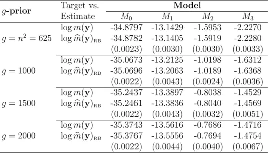
discussed in Section 2.5 using estimator (7) and the model with g = 1000 as the base model from which we sample from the posterior 10,000 draws discarding the first 1000 as burn-in. Batch mean estimates from the Rao-Blackwell estimator and MC errors, based on 30 batches 300 draws, along with the true marginal log-likelihoods are presented in Table 2.
g-prior Target vs. Model
Estimate M0 M1 M2 M3 g =n2 = 625 logm(y) -34.8797 -13.1429 -1.5953 -2.2270 logmb(y)RB -34.8782 -13.1405 -1.5919 -2.2280 (0.0023) (0.0030) (0.0030) (0.0033) g = 1000 logm(y) -35.0673 -13.2125 -1.0198 -1.6312 logmb(y)RB -35.0696 -13.2063 -1.0189 -1.6368 (0.0022) (0.0043) (0.0024) (0.0036) g = 1500 logm(y) -35.2437 -13.3897 -0.8038 -1.4529 logmb(y)RB -35.2461 -13.3836 -0.8040 -1.4569 (0.0022) (0.0043) (0.0032) (0.0051) g = 2000 logm(y) -35.3743 -13.5616 -0.7686 -1.4716 logmb(y)RB -35.3767 -13.5556 -0.7694 -1.4754 (0.0022) (0.0044) (0.0040) (0.0067)
Table 2: Estimated marginal log-likelihood Rao-Blackwell estimates compared with the true values for Example 1 for the initial g-prior and three diffuse g-priors for the regression vector; average batch mean estimates (MC errors in parentheses) are presented using 30 batches of size 300. The estimates for g = 1500 and g = 2000 are based on posterior samples from the models withg = 1000.
As seen in Table 2, the estimates are accurate despite the fact that the posterior distributions remain the same. In addition, using estimator (7) based on draws from the model withg = 1000 required only calculation of prior probabilities for the models withgequal to 1500 and 2000, and led to consistent marginal likelihood estimates. The estimates based on the exact marginal posteriors (not presented here) are equivalent.
3.2
Finite normal mixture models
In this example we consider the well-known galaxy data which where initially presented by Postman et al. (1986). The data are velocities (km’s per second) of 82 galaxies from six separated conic sections of the Corona Borealis region. The data set is taken fromMASSlibrary in R which contains a “typo”; the value of the 78th observation was
corrected to 26960. The goal is to investigate whether the galaxies can be classified into different clusters according to their velocities, as suggested in astronomical theories. Gaussian finite mixture models are used in the related literature with the purpose of finding the most plausible number of clusters or components. Under this modeling assumption, the likelihood of the velocity datay= (y1, y2, ..., yn)T for a model withk
componentswj ∈(0,1), such that Pjwj = 1 for j = 1,2, ..., k, is given by
l(y|µ,σ2,w) = n Y i=1 k X j=1 wjφ(yi|µj, σ2j), (10) where w = (w1, w2, ..., wk)T, µ = (µ1, µ2, ..., µk)T, σ2 = (σ12, σ22, ..., σk2)T and φ(·) is
the p.d.f. of the normal distribution. Vectors µ and σ2 consist of the component-specific means and variances, respectively. As originally shown in Dempster et al. (1977), any mixture model can be expressed in terms of missing or latent data; if
zi ∈ {1,2, ..k}represents a latent indicator variable associated with observation yi, so
that Pr(zi =j) =wj and l(yi|zi =j, µj, σj2) =φ(yi|µj, σj2), then we have that
l(yi, zi =j|µj, σj2) = l(yi|zi =j, µj, σ2j) Pr(zi =j) =φ(yi|µj, σj2)wj.
Summation over the components wj results in the complete marginalized data
likeli-hood presented in (10).
As illustrated in West (1992) and Diebolt and Robert (1994), data-augmentation facilitates posterior simulation via Gibbs sampling from the full conditional densities of w,µ,σ2 and z. The conjugate priors areµ
j ∼ N(µ0, σ02),σj2 ∼IG(ν0/2, δ0/2) and
w∼Dir(α1, α2, ..., αk). The prior forzis fixed by model design, since Pr(zi =j) =wj.
Gibbs sampling is straightforward to implement, given these prior assumptions; let
Tj = {i : zi = j} be the set of observation indices for those yi classified into the
j-th cluster and letnj denote the number of observations falling into the j-th cluster.
Then, we sample sequentially
zi|y, µj, σj2, wj ∼ Pr(zi =j|y, wj, µj, σj2)∝wjφ(yi|µj, σ2j), µj|y, σj2,z ∼ N(µbj,bs 2 j), σj2|y, µj,z ∼ IG ν 0+nj 2 , δ0+δj 2 , w|y,z ∼ Dir(α1+n1, α2+n2, ..., αk+nk), whereµbj =bs 2 j(σ −2 0 µ0+σj−2 P i∈Tjyi),bs 2 j = (σ −2 0 +σ −2 j nj)−1 and δj = P i∈Tj(yi−µj) 2.
We are also interested in models which have a common variance term in (10); in this case the full conditional of σ2 is IG(ν0+n
2 , δ0+δ 2 ) with δ = Pk j=1 P i∈Tj(yi−µj) 2.
A central point in the discussion that follows is the identifiability problem which is present in mixture models, known as “label-switching”. Non-identifiability arises from the fact that relabelling the mixture componentswj does not change the likelihood in
distribution has k! symmetrical modes. In terms of posterior sampling this implies that common MCMC samplers will most probably fail to explore adequately all k! modes as it is very likely that an MCMC chain will get “trapped” in one particular mode thus leaving the remaining k!−1 modes unvisited. A first suggestion proposed in the early literature is to impose prior ordering constraints, e.g. w1 < w2 < ... < wk
or µ1 < µ2 < ... < µk, which translate to truncated priors that restrict inference to
constrained unimodal posteriors. Robert and Mengersen (1999) further extended this strategy to the use of improper priors through reparameterization. Nevertheless, other authors object to the use of prior identifiability constraints and recommend sampling from the unconstrained posterior. Among them, Celeux et al. (2000) propose tem-pered transition algorithms and appropriate loss functions for permutation invariant posteriors, while Marin et al. (2005) suggest ex-post reordering schemes.
Chib (1995) was the first who estimated directly the marginal likelihoods of these data for two and three component models via the candidate’s formula and Gibbs up-dating for the estimation of reduced posterior ordinates. Nevertheless, as pointed out in Neal (1998), Chib’s use of the Gibbs sampler for mixture models results in biased marginal likelihood estimates due to lack of label-switching within the Gibbs sampler. A simple approach to correct for bias is to multiply the marginal likelihood estimates with a factor ofk!, but as Neal remarked the bias correction will only be valid when the symmetrical modes are well-separated (i.e. when label-switching is not likely to oc-cur). Therefore, Neal (1998) suggests either to introduce special relabelling transitions into the Gibbs sampler or to enforce constrained priors during Gibbs updating which will be k! times larger than the unconstrained priors, as general but computationally demanding solutions. Motivated by the practical bias-correction approach, Berkhof et al. (2003) present simulation consistent marginal likelihood estimators based on a stratification principle and ex-post randomly permuted samples. Fr¨uhwirth-Schnatter (2004), on the other hand, recommends to use MCMC samplers which adequately explore all k! labeling posterior subspaces and presents bridge-sampling estimators based on draws from the unconstrained random permutation sampler introduced in Fr¨uhwirth-Schnatter (2001).
We consider the same models as Chib (1995) and show that the estimator proposed here can accurately estimate the marginal likelihoods either by taking into account the bias-correction of Neal (1998) or through the use of MCMC samplers which ex-plore effectively the unconstrained posterior space. Specifically, interest lies in the 2-component equal-variance model and 3-component models with equal and unequal variances (i.e. k = 2,3), under the prior assumptions µ0 = 20, σ02 = 100, ν0 = 6,
δ0 = 40 and αj = 1 for j = 1,2, ..., k. We further take into account a 4-component
equal variance model (k = 4) with the same prior assumptions. Models with more than four clusters are not considered due to the fact that there is not enough infor-mation in the data to supportk >3, which gives rise to serious convergence problems due to non-identifiability of parameters for more than four clusters; see Carlin and Chib (1995).
bayesmix (Gr¨un, 2011) in R, which also allows for ex-post reordering and random permutation sampling. We iterate the Gibbs sampler 13,000 times and discard the first 1000 iterations as burn-in. In the context of Section 2 this is a multi-block problem (θ1 ≡µ,θ2 ≡σ2,θ3 ≡w), including a latent vector (u≡z) which is integrated out.
We divide the reordered product marginal posterior sample into K = 30 batches of
NK = 400 draws and calculate the marginal likelihood for each batch as
b m(y) =NK−1 NK X n=1 l(y|µ(n),σ2(n),w(n))π(µ(n))π(σ2(n))π(w(n)) p(µ(n)|y)p(σ2(n)|y)p(w(n)|y) .
Marginal posterior densities are estimated through Rao-Blackwellization based on re-duced samples of sizeL= 500, i.e. p(µ|y)=Q
j 1 L PL l=1p(µj|y, σ 2(l) j ,z(l)) ,p(σ2|y) =Q j 1 L PL l=1p(σ 2 j|y, µ (l) j ,z (l)) and p(w|y) = L1 PL l=1p(w|y,z (l)), for j = 2,3,4. For
the equal-variance models we have that p(σ2|y) = 1
L PL
l=1p(σ2|y, µ (l)
j ,z(l)). Table 3
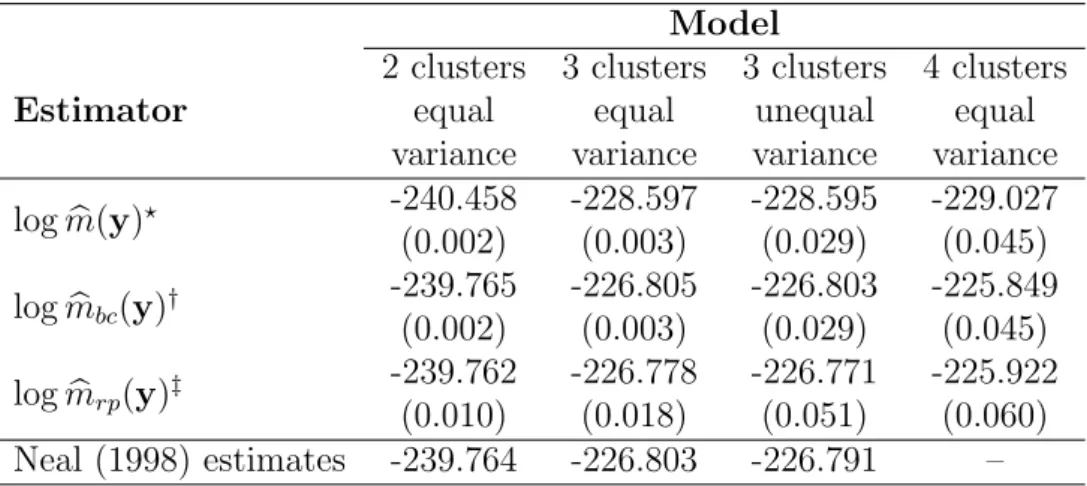
shows batch mean estimates on log scale and the corresponding MC errors for the simple estimator mb(y), the bias-corrected estimator mbbc(y) (obtained by adding the
constant logk! to logmb(y)) and the estimator based on ex-post random permutation sampling mbrp(y).
Model
2 clusters 3 clusters 3 clusters 4 clusters
Estimator equal equal unequal equal variance variance variance variance
logmb(y)? -240.458 -228.597 -228.595 -229.027 (0.002) (0.003) (0.029) (0.045) logmbbc(y)† -239.765 -226.805 -226.803 -225.849 (0.002) (0.003) (0.029) (0.045) logmbrp(y)‡ -239.762 -226.778 -226.771 -225.922 (0.010) (0.018) (0.051) (0.060) Neal (1998) estimates -239.764 -226.803 -226.791 – ? b
m(y): Simple (biased) estimator; †mbbc(y): Bias-corrected estimator;
‡
b
mrp(y): Random
permutation sampling estimator.
Table 3: Estimated marginal log-likelihood values for Example 2; average batch mean estimates (MC errors in parentheses) are presented using 30 batches of size 400.
The benchmark results reported by Neal (1998), based on 108 draws from the
prior distributions, are also included in Table 3; the corresponding standard errors are 0.005 for the 2 component equal-variance model, 0.040 for the three component equal-variance model and 0.089 for the three component unequal-variance model. It is obvious, that the simple estimatormb(y) results in biased estimates, which are very similar to the ones presented in Chib (1995); see Neal (1998) for the “typo-corrected” estimate of Chib for the 3rdmodel. On the other hand, as reflected in the bias-corrected
estimates which are in agreement with the estimates of Neal. Interestingly, the MC errors ofmbbc(y) are similar to the “coefficients of variation” in Steele et al. (2006) who
handle marginal likelihood estimation through an incremental mixture importance sampling approach based on marginalization. Nevertheless, Steele et al. (2006) adopt different prior assumptions and, therefore, their marginal likelihood estimates are not comparable to the ones in Table 3.
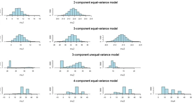
Figure 1: Histograms of posterior means for the three models from Gibbs sampling. Histograms of posterior means from Gibbs sampling are presented in Figure 1. As seen, the Gibbs sampler remains in one particular mode for the 2-component and 3-component equal variance models. This is not the case for the 3-component unequal variance model, where label-switching does actually occur for parameters µ1
and µ2. For the 4-component model label-switching is noticeable for all posterior
means. Despite that fact, the bias-corrected estimator still performs well for these models. Nevertheless, we would not warrant to guarantee that the bias-corrected estimator will always perform well, especially as the number of clusters gets larger and the posterior modes are not well separated.
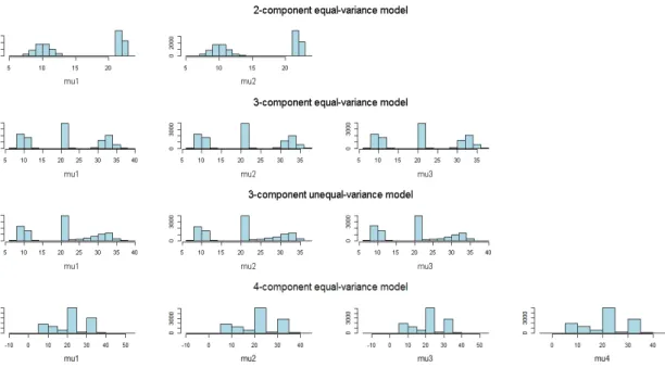
Alternatively, one can simply use random permutation sampling and estimate the marginal likelihoods without the need to account for bias-correction. In addition, random permutation sampling will probably prove to be a more reliable solution for models with many components, since the marginal posteriors from random permu-tation sampling capture all possible modes. The estimates from mbrp(y) are indeed
very similar to Neal’s estimates and to the bias-corrected estimates. The MC errors are slightly higher for the random permutation estimates, nevertheless, this is under-standable since ex-post random permutation artificially increases MCMC variability. Histograms of posterior means from random permutation sampling are presented in
Figure 2: Histograms of posterior means for the three models from random permuta-tion sampling.
Figure 2; the symmetries in the posterior distributions due to non-identifiability are now apparent. In accordance to the discussion in Carlin and Chib (1995), the his-tograms for the 4-component model show that only three modes are estimated effi-ciently as there is a significant overlap between the 2nd and 3rd mode.
In conclusion, both mbbc(y) andmbrp(y) yield satisfactory results. For models with
a small number of components (i.e. when label-switching is not likely to occur) the bias-corrected estimator will most probably be sufficient. For more complicated mod-els and when the two estimators result in estimates which are in disagreement, we would recommend to use either the correction for the candidate estimator proposed by Marin and Robert (2008) or the estimator based on alternative MCMC strategies (e.g. Fr¨uhwirth-Schnatter, 2001; Geweke, 2007).
3.3
Longitudinal Poisson models
As a last example, we consider a data set taken from Diggle et al. (1995), consisting of seizure counts yit from a group of epilepticts (i = 1,2, ...,59) which is monitored
initially over an 8-week baseline period (t= 0) and then over four subsequent 2-week periods (t = 1,2,3,4). Each patient is randomly assigned either a placebo or the drug progabide after the baseline period. This example is chosen mainly because standard Gibbs sampling is not possible to implement for the model presented next. In addition, the epilepsy data is also considered by Chib et al. (1998) and Chib and Jeliazkov (2001) who present marginal likelihood estimates based on the candidate’s formula and Metropolis-Hastings sampling. Reduced posterior ordinates are calculated through
kernel density estimation in Chib et al. (1998), whereas Chib and Jeliazkov (2001) employ Metropolis-Hastings updating. For the sake of comparison, we adopt exactly the same modeling assumptions.
The main model under consideration is
yit|β,bi ∼ Poisson(λit),
logλit = logτit+β1xit1+β2xit2 +bi1+bi2xit2,
bi ∼ N2(η,D),
where τit is the offset which equals 8 when t= 0 and 2 otherwise, xit1 is an indicator
of treatment (0 for placebo, 1 for progabide treatment), xit2 is an indicator of time
period (0 for baseline, 1 otherwise) and bi = (bi1, bi2) are latent random effects for
i= 1,2, ...,58 (subject 49 is removed from the analysis due to unusually high pre-and post-randomization seizure counts). The prior assumptions are bivariate normal distri-butions forβ andη and a bivariate inverse-Wishart for D, namely β∼ N2(0,100I2),
η ∼ N2(0,100I2) and D ∼ IW2(4,I2), where I2 is the 2×2 identity matrix. The
full conditionals ofη and D are known, specifically we have that
η|D,b1, ...,b58 ∼ N2(ηb,V), D|η,b1, ...,b58 ∼ IW2 58 + 4,I2+ 58 X i=1 (bi−η)(bi−η)T , where ηb = VP58 i=1D −1b
i and V = (100−1I2 + 58D−1)−1. The full
condition-als for β and the bi’s are not known distributions and thus standard Gibbs
sam-pling is not feasible. Another complication is that the integrated samsam-pling likelihood
l(y|β,η,D) = Q58 i=1
R
l(yi|β,bi)π(bi)dbi, with l(yi|β,bi) = Q4t=0l(yit|β,bi), is also
not available analytically. Therefore, evaluating l(y|β,η,D) requires either numer-ical integration or some other efficient technique, such as importance sampling for instance.
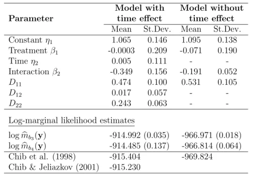
We utilize WinBUGS software (Spiegelhalter et al., 2003) to sample from the posterior. Specifically, one chain is iterated 31,000 times and the first 1000 iterations are discarded as burn-in, resulting in a final sample of 30,000 draws. Posterior means and standard deviations, for the parameters of scientific interest, are presented in Table 4. The estimates for the main model are comparable to the Metropolis-Hastings estimates presented in Chib et al. (1998). Table 4 also includes the estimates for the simpler model without the random effects related to time. For this model we assume a-priori that bi ∼ N(η1, D11), for i = 1,2, ...,58. In order to keep equivalent
prior assumptions to the main model, we define the priors as η1 ∼ N(0,100) and
D11 ∼ IG(2,1/2).
As discussed in Section 2.3, there are two approaches for estimating the marginal likelihood of this model. The first is to treat it as a 3-block setting, i.e. consider the product of the marginal posteriors of β,η,D as importance sampling density. In this case one needs to estimate the integrated likelihood which is unknown. The
second approach is to treat the problem as a 4-block setting, i.e. also include the joint marginal posterior of thebi’s in the importance sampling density. The advantage with
this approach is that we can work directly with the hierarchical Poisson likelihood. Initially, let us consider the first approach which corresponds to estimator (5) of Section 2.3; in this case the parameters of scientific interest are θ1 ≡ β,θ2 ≡
η,θ3 ≡ D, while u ≡ {b1, ...,b58} is used only for Rao-Blackwellization. First, we
appropriately re-order the posterior sample in order to correspond to a sample from the product marginal posterior and then we split the sample into K = 30 batches of
NK = 1000 draws. The marginal likelihood estimate for each batch is calculated as
b mb3(y) =N −1 K NK X n=1 l(y|β(n),η(n),D(n))π(β(n) )π(η(n))π(D(n)) p(β(n)|y)p(η(n)|y)p(D(n)|y) .
Marginal posterior probabilities for η and D are estimated via Rao-Blackwellization based on reduced posterior samples ofL= 200 draws which are randomly re-sampled from the initial MCMC sample, i.e. p(η|y)=1
L PL l=1p(η|D (l),b(l) 1 , ...,b (l) 58) andp(D|y) = 1 L PL l=1p(D|η (l),b(l) 1 , ...,b (l)
58). For the marginal posterior ofβwe assume thatp(β|y)≈
N2( ˜β,Σ˜), where ˜β and ˜Σ are estimated from the MCMC output. Similarly to Chib
et al. (1998) and Chib and Jeliazkov (2001), we employ further importance sampling to evaluate the likelihood l(y|β,η,D). We employ multivariate normals as impor-tance sampling functions, namely pIS(b1, ...,b58|y) ≈ N116(˜b,B˜) for the main model
and pIS(b1, ..., b58|y)≈ N58(˜b,B˜) for the reduced model, where ˜b,B˜ are the vector of
means and the complete covariance matrix of the random effects estimated from the MCMC output. Likelihood estimation is based on 100 importance sampling draws.
Based on the alternative 4-block approach, corresponding to estimator (6) of Sec-tion 2.3, the batched marginal likelihood estimates are calculated as
b mb4(y) =N −1 K NK X n=1 l(y|β(n),b1(n), ...,b(58n))× π(β(n))π(b1(n), ...,b(58n)|η(n),D(n))π(η(n))π(D(n))× n p(β(n)|y)p(b(1n), ...,b58(n)|y)p(η(n)|y)p(D(n)|y) o−1 .
With this approach, there is no need to implement further importance sampling for evaluating the likelihood function since the data conditional on the random effects pa-rameters follow the Poisson distribution. Despite this convenient aspect, the downside of the 4-block estimator is that it requires estimation of the high-dimensional joint marginal p(b1, ...,b58|y). Given that the Rao-Blackwell device cannot be used, we
adopt a simple assumption and namely use the importance sampling functions used for likelihood evaluation in estimator mbb3(y), i.e. we assume that p(b1, ...,b58|y) ≈
N116(˜b,B˜) for the model with time effects and p(b1, ..., b58|y) ≈ N58(˜b,B˜) for the
model not including time effects.
Average batch mean marginal likelihood estimates and MC errors for the two models in question are presented in Table 4. The 3-block approach provides accurate
Parameter
Model with Model without time effect time effect
Mean St.Dev. Mean St.Dev.
Constantη1 1.065 0.146 1.095 0.138 Treatment β1 -0.0003 0.209 -0.071 0.190 Time η2 0.005 0.111 - -Interaction β2 -0.349 0.156 -0.191 0.052 D11 0.474 0.100 0.531 0.105 D12 0.017 0.057 - -D22 0.243 0.063 -
-Log-marginal likelihood estimates
logmbb3(y) -914.992 (0.035) -966.971 (0.018) logmbb4(y) -914.485 (0.137) -966.814 (0.064)
Chib et al. (1998) -915.404 -969.824
Chib & Jeliazkov (2001) -915.230
Table 4: Posterior means and standard deviations from 30,000 posterior draws for the parameters of two epilepsy models and average batch mean marginal likelihood estimates (MC errors in brackets) from 30 batches of size 1000 for the 3-block and 4-block estimators for Example 3.
estimates with MC errors being very low in comparison to the magnitude of the batched means. The 4-block estimates are in agreement with the 3-block estimates, but have higher Monte Carlo errors; approximately four times higher than the MC errors of mbb3(y). Nevertheless, this is expected due to the much larger augmented parameter space and the use of the normal approximation of the high-dimensional joint posterior of the random effects. Overall, estimatormbb4(y) is computationally less demanding than mbb3(y) and the resulting MC errors, although higher than those of
b
mb3(y), are still relatively low in comparison to the batched mean marginal likelihood values.
Table 4 also includes the estimates presented in Chib et al. (1998) and Chib and Jeliazkov (2001) from 10,000 posterior draws. Both latter studies report standard errors, based on the variance estimator of Newey and West (1987), of approximately 0.1 for the main model. The reduced model is briefly considered in Chib et al. (1998) without reporting a standard error. Our 3-block and 4-block estimates are compa-rable to those of Chib et al. (1998) and Chib and Jeliazkov (2001) but not in strict agreement. Our experience from this particular example is that a long MCMC chain is needed in order to obtain accurate posterior estimates; initial 3-block estimates based on 10,000 posterior draws were actually closer to the estimates of Chib et al. (1998) and Chib and Jeliazkov (2001), namely -915.566 for the main model and -969.580 for the reduced model, but with considerably higher MC errors.
3.4
MC errors for different number of iterations
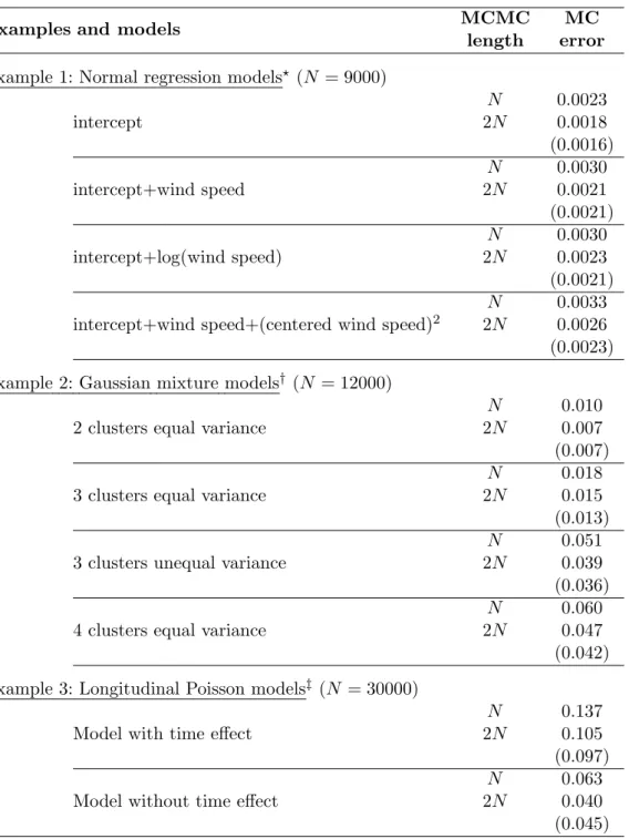
Here we briefly investigate the issue of finite variance for the illustrated examples presented in this section. Following the discussion in Section 2.6, an informal empirical
Examples and models MCMC MC
length error
Example 1: Normal regression models? (N = 9000) intercept N 0.0023 2N 0.0018 (0.0016) intercept+wind speed N 0.0030 2N 0.0021 (0.0021) intercept+log(wind speed) N 0.0030 2N 0.0023 (0.0021) intercept+wind speed+(centered wind speed)2
N 0.0033
2N 0.0026
(0.0023) Example 2: Gaussian mixture models† (N = 12000)
2 clusters equal variance
N 0.010
2N 0.007
(0.007) 3 clusters equal variance
N 0.018
2N 0.015
(0.013) 3 clusters unequal variance
N 0.051
2N 0.039
(0.036) 4 clusters equal variance
N 0.060
2N 0.047
(0.042) Example 3: Longitudinal Poisson models‡ (N = 30000)
Model with time effect
N 0.137
2N 0.105
(0.097) Model without time effect
N 0.063
2N 0.040
(0.045) ?MC errors for the Rao-Blackwell estimator forg=n2;†MC errors for the random permutation
estimator;‡MC errors for the 4-block estimator
Table 5: MC errors of marginal log-likelihood estimates for MCMC runs of length
N and 2N; the number of batches is 30 for all models. The expected MC errors for samples of size 2Nunder the assumption of finite variance are presented in parentheses.
diagnostic for checking whether the variance is finite can be performed by comparing the MC errors from MCMC samples of different sizes. In general, increasing the MCMC sample by a factor of d should lead to a decrease of MC errors by a factor of √d for estimators which have finite variance. Table 5 depicts the estimated MC errors for the Rao-Blackwell estimator for Example 1, the estimator based on random-permutation sampling for Example 2 and the 4-block estimator for Example 3. In all cases, the MC errors from the original posterior samples of sizeN are compared with the corresponding errors from samples of size 2N and with the errors from the original samples scaled down by a factor of√2, which are the expected MC errors under the assumption of finite variance. From this table, it is evident that the MC errors from the MCMC runs with length equal to 2N are roughly equal to the MC errors from the chains with length N divided by √2, for all models, indicating that the variance of the corresponding estimators is finite.
4
Concluding remarks
In this paper we have presented a method of marginal likelihood estimation based on utilizing the product marginal posterior as importance sampling density. The approach is in general straightforward to implement even for multi-block parameter settings as it is non-iterative and does not require adaptations in MCMC sampling. As illustrated, the estimator is accurate in capturing changes in the marginal likelihood due to different diffuse prior setups that do not affect the posterior distribution. For such cases, the computational demands for estimating marginal likelihoods of com-peting models under diffuse priors are reduced significantly, since only one MCMC run is required. In general, the overall performance of the estimator depends on; i) the efficiency of approximating the joint posterior through independent univariate or multivariate marginals and ii) the accuracy in estimating marginal posterior densities. Arguably, the method can fail when the product of marginal posteriors is a poor approximation to the joint posterior. Nevertheless, appropriate parameter blocking and reparameterizations can always improve the performance of the method, so that it will be feasible to work with a few parameter blocks that are close to orthogonal regardless whether the elements within the blocks are highly correlated. In the three, relatively diverse, examples handled in this paper the natural blocking of the param-eters proved to be sufficient in delivering accurate estimates. It is worth noting that similar estimators based on importance sampling from independent posterior factor-izations have shown to perform well (Botev et al., 2012; Chan and Eisenstat, 2013). Moreover, independent posterior factorization is also extensively used for the varia-tional Bayes (Bishop, 2006) and expectation-propagation (Minka, 2001) approaches in the maching-learning literature. As a last remark concerning this topic, Ghosh and Clyde (2011) present a methodology for linear and binary regression models that aug-ments non-orthogonal designs to obtain orthogonal designs based on Gibbs sampling for the “missing” response variables. With some additional effort one could consider
this orthogonalization approach which would guarantee an optimal importance sam-pling density, thus leaving estimation of univariate marginal posterior densities as the only remaining source of error.
With respect to estimating marginal probabilities, the approach proposed here is particularly suited for Gibbs sampling settings where Rao-Blackwellization can be used to obtain simulation-consistent marginal posterior density estimates. Practi-cally, the proposed estimator can get computationally demanding when using Rao-Blackwellization for the entire posterior sample. Nevertheless, the related coding work basically requires averaging and is straighforward, without requiring any special effort in implementation or fine-tuning of parameters in trial and error runs. In ad-dition, as illustrated in the examples, the sample needed for Rao-Blackwellization is substantially smaller than the total MCMC sample and is obtained once as a random sub-sample of the MCMC chain.
The approach can also be applied under other types of MCMC schemes by adopt-ing other strategies for estimatadopt-ing the marginal posterior densities such as normal approximations, fitting posterior moments, kernel methods and so forth. In strict theory, the method will not yield unbiased estimates when using such approximating strategies, nevertheless, in practical terms such approaches can often be sufficient and can lead to accurate estimates even for high dimensional multivariate approximations, as demonstrated in Section 3.3. In addition, the degree of bias can be checked in-directly by using the approximating densities as importance sampling densities. It is worth noting, that more elaborated strategies can also be considered, for instance the methods discussed in Oh (1999) based on importance-weighted marginal density estimation (Chen, 1994) or the integrated nested Laplace approximations (INLA’s) presented in Rue et al. (2009).
The advantage of not depending on the type of MCMC scheme used to sample from the posterior becomes obvious for classes of models like the finite normal mixtures, considered here, where conventional Gibbs sampling fails to explore multi-modal pos-terior surfaces. This implies that the proposed method will also work well for models with similar posterior symmetries, based on alternative samplers (e.g. Fr¨ uhwirth-Schnatter, 2001; Geweke, 2007), without increased complexity in estimation.
A possibly interesting extension of the idea presented here is to incorporate it within bridge-sampling estimation by using the product marginal posterior as approx-imating density.
Acknowledgements
The authors would like to thank two anonymous referees for their interesting comments and suggestions.
References
Ardia, D., Ba¸st¨urk, N., Hoogerheide, L. and van Dijk, H.K. (2012). A compara-tive study of Monte Carlo methods for efficient evaluation of marginal likelihood.
Computational Statistics and Data Analysis, 56, 3398–3414.
Berkhof, J., van Mechelen, I. and Gelman, A. (2003). A Bayesian approach to the selection and testing of mixture models. Statistica Sinica,13, 423–442.
Bishop, C.M. (2006).Pattern Recognition and Machine Learning. New York: Springer. Botev, Z., L’Ecuyer, P. and Tuffin, B. (2013). Markov chain importance sampling with applications to rare event probability estimation. Statistics and Computing,
23, 271–285.
Carlin, B.P. and Chib, S. (1995). Bayesian model choice via Markov chain Monte Carlo methods. Journal of the Royal Statistical Society B, 57, 473–484.
Carlin, B.P. and Louis, T. (1996). Bayes and Empirical Bayes Methods for Data Analysis. London: Chapman & Hall\CRC.
Celeux, G., Hurn, M. and Robert, C. (2000). Computational and inferential diffi-culties with mixtures posterior distribution. Journal of the American Statistical Association, 95, 957–979.
Chan, J. and Eisenstat, E. (2013). Marginal likelihood estimation with the cross-entropy method. Econometric Reviews, forthcoming.
Chen, M.-H. (1994). Importance-weighted marginal Bayesian posterior density esti-mation. Journal of the American Statistical Association, 89, 818–824.
Chen, M.-H. (2005). Computing marginal likelihoods from a single MCMC output.
Statistica Neerlandica, 59, 16–29.
Chib, S. (1995). Marginal likelihood from the Gibbs output. Journal of the American Statistical Association, 90, 1313–132.
Chib, S., Greenberg, E. and Winkelmann, R. (1998). Posterior simulation and Bayes factors in panel count data models. Journal of Econometrics, 86, 33–54.
Chib, S. and Jeliazkov, I. (2001). Marginal likelihood from the Metropolis-Hastings output. Journal of the American Statistical Association, 96, 270–281.
Dellaportas, P., Forster, J.J. and Ntzoufras, I. (2002). On Bayesian model and variable selection using MCMC. Statistics and Computing, 12, 27–36.
Del Moral, P., Doucet, A. and Jasra, A. (2006). Sequential Monte Carlo samplers.
Dempster, A. P., Laird, N. M. and Rubin, D. B. (1977). Maximum likelihood from incomplete data via the EM algorithm (with discussion). Journal of the Royal Statistical Society B, 39, 1–38.
Diebolt, J. and Robert, C.P. (1994). Estimation of finite mixture distributions through Bayesian sampling. Journal of the Royal Statistical Society B, 56, 363–375.
Diggle, P., Liang, K.-Y. and Zeger, S.L. (1995).Analysis of Longitudinal Data. Oxford: Oxford University Press.
Fern´andez, C., Ley, E. and Steel, M.F.J. (2001). Benchmark priors for Bayesian model averaging. Journal of Econometrics, 100, 381–427.
Feroz, F., Balan, S.T. and Hobson, M.P. (2011). Bayesian evidence for two compan-ions orbiting HIP 5158. Monthly Notices of the Royal Astronomical Society, 416, L104–L108.
Feroz, F., Hobson, M.P. and Bridges, M. (2009). MULTINEST: an efficient and robust Bayesian inference tool for cosmology and particle physics. Monthly Notices of the Royal Astronomical Society, 398, 1601–1614.
Friel, N. and Pettitt, A.N. (2008). Marginal likelihood estimation via power posteriors.
Journal of the Royal Statistical Society B, 70, 589–607.
Friel, N. and Wyse, J. (2012). Estimating the evidence – a review. Statistica Neer-landica, 66, 288–308.
Fr¨uhwirth-Schnatter, S. (2001). Markov chain Monte Carlo estimation of classical and dynamic switching and mixture models. Journal of the American Statistical Association, 96, 194–209.
Fr¨uhwirth-Schnatter, S. (2004). Estimating marginal likelihoods for mixture and Markov switching models using bridge sampling techniques. The Econometrics Journal,7, 143–167.
Gelfand, A.E. and Smith, A.F.M. (1990). Sampling-based approaches to calculating marginal densities. Journal of the American Statistical Association, 85, 398–409. Gelman, A. and Rubin, D.B. (1992). Inference from iterative simulation using multiple
sequences. Statistical Science, 7, 457–511.
Geweke, J. (2007). Interpretation and inference in mixture models: simple MCMC works. Computational Statistics and Data Analysis, 51, 3529–3550.
Geyer, C.J. (1992). Practical Markov chain Monte Carlo. Statistical Science, 4, 473–483.
Ghosh, J. and Clyde, M.A. (2011). Rao-Blackwellization for Bayesian variable selec-tion and model averaging in linear and binary regression: a novel data augmentaselec-tion approach. Journal of the American Statistical Association, 106, 1041–1052.
Gilks, W.R. and Roberts, G.O. (1996). Strategies for improving MCMC. In Markov Chain Monte Carlo in Practice, 6, eds. W.R. Gilks, S. Richardson and D.J. Spiegel-halter, London: Chapman & Hall\CRC, pp. 89–114.
Green, P.J. (1995). Reversible jump Markov chain Monte Carlo computation and Bayesian model determination. Biometrika,82, 711–732.
Gr¨un, B. (2011). bayesmix: Bayesian Mixture Models with JAGS. Available at http://cran.r-project.org/web/packages/bayesmix/index.html.
Kass, R.E. and Raftery, A.E. (1995). Bayes factors and model uncertainty. Journal of the American Statistical Association, 90, 773–795.
Lewis, S.M. and Raftery, A.E. (1997). Estimating Bayes factors via posterior simu-lation with the Laplace-Metropolis estimator. Journal of the American Statistical Association, 92, 648–655.
Marin, J.-M., Mengersen, K. and Robert, C. (2005). Bayesian modelling and inference on mixtures of distributions. In Handbook of Statistics, vol. 25, eds. C. Rao and D. Dey, New York: Elsevier, pp. 459–507.
Marin, J.-M and Robert, C.P. (2008). Approximating the marginal likelihood in mixture models. Bulletin of the Indian Chapter of ISBA, V(1), 2–7; also available as arXiv0804.2414.
Meng, X.-L. and Wong, W.H. (1996). Simulating ratios of normalizing constants via a simple identity: a theoretical exploration. Statistica Sinica, 6, 831–860.
Minka, T.P. (2001). Expectation propagation for approximate Bayesian inference.
Uncertainty in Artificial Intelligence, 17, 362–369.
Montgomery, D.C., Peck, E.A. and Vining, G.G. (2001). Introduction to Linear Re-gression Analysis. New York: John Wiley.
Neal, R.M. (1998). Erroneous results in ‘Marginal likelihood from the Gibbs output’. Available at http://www.cs.utoronto.ca/radford/[email protected].
Neal, R.M. (2001). Annealed importance sampling. Statistics and Computing, 11, 125–139.
Newey, W. K. and West, K. D. (1987). A simple positive semi-definite heteroskedas-ticity and autocorrelation consistent covariance matrix. Econometrica,55, 703–708.