Active Learning for Data Streams Under Concept Drift and
Concept Evolution
Saad Mohamad?, Moamar Sayed-Mouchaweh, and Abdelhamid Bouchachia Ecole des Mines, Douai, France
Bournemouth University, Poole, UK
{saad.mohamad,moamar.sayed-mouchaweh}@mines-douai.fr {smohamad,abouchachia}@bournemouth.ac.uk
Abstract. Data streams classification is an important problem however, poses many chal-lenges. Since the length of the data is theoretically infinite, it is impractical to store and process all the historical data. Data streams also experience change of its underlying dis-tribution (concept drift), thus the classifier must adapt. Another challenge of data stream classification is the possible emergence and disappearance of classes which is known as ( con-cept evolution) problem. On the top of these challenges, acquiring labels with such large data is expensive. In this paper, we propose a stream-based active learning (AL) strategy (SAL) that handles the aforementioned challenges. SAL aims at querying the labels of samples which results in optimizing the expected future error. It handlesconcept drift and concept evolutionby adapting to the change in the stream. Furthermore, as a part of the error reduc-tion process, SAL handles thesampling biasproblem and queries the samples that caused the change i.e., drifted samples or samples coming from new classes. To tackle the lack of prior knowledge about the streaming data, non-parametric Bayesian modelling is adopted namely the two representations of Dirichlet process; Dirichlet mixture models and stick breaking process. Empirical results obtained on real-world benchmarks show the high performance of the proposed SAL method compared to the state-of-the-art methods.
Keywords: Data Streams, Active Learning, Concept Drift, Concept Evolution, Novelty detection.
1
Introduction
Classification has been the focus of a large body of research due to its key relevance to numerous real-world applications. A classifier is trained by learning a mapping function between input and pre-defined classes. In an offline setting, the training of a classifier assumes that the training data is available prior to the training phase. Once this latter is exhausted, the classifier is deployed and, cannot be trained any further even if performs poorly. This can happen if the training data used does not exhibit the true characteristics of the underlying distribution. Moreover, for many applications data arrives over time as a stream and therefore the offline assumptions cannot hold. Data streams classification presents many challenges because of the continuous and evolving nature of streams, in addition to the problem of labelling of such large data.
Data streams are assumed to be unbounded in size, which makes it infeasible to store all the data to train the proposed model. Hence, online learning algorithms must be used [1–6].
Data streams may evolve over time so that the relationship between the input data instances and their labels changes, leading to what is known asconcept drift [7, 8]. Thus, to deal with data streams classification efficiently, the classifier must (self-)adapt online over time [1, 9–11].
The evolving nature of data streams poses another challenge which is rarely addressed in the literature and known as concept evolution. This occurs when a new classes emerge or existing classes vanish. The classifier must be able to identify the new classes and incorporate them into the decision model [12–15]. Emergence of new classes has been studied in the context of novelty detection, where the task is to identify the outlier instances. This is seen asone-class classification, in which a very large number of data samples describingnormal condition is available while the data samples describing theabnormalitiesare rare [16, 17]. In contrast,Concept evolution involves the emergence of different normal and abnormal classes.
Given the large volume and high velocity of data streams, it is impractical to acquire the label of each instance. Active learning (AL) is a promising way to efficiently building up training sets
with minimal supervision. AL deliberately queries particular instances to train the classifier using as few labelled data instances as possible. AL for data streams is more challenging because both concept drift and concept evolution can occur at any time and anywhere in the feature space. Another challenge associated with AL, in general, is the sampling bias [18] where the sampled training set does not reflect the underlying data distribution in a destructive way. Basically, AL seeks to query samples which labelling them significantly improves the learning. That is instead of sampling from the data underlying distribution, AL deliberately creates a bias training set. However, as AL becomes increasingly confident about its sampling assessment, valuable samples could be ignored and the bias of the training set could become harmful.
In this paper, we propose an AL algorithm, called Stream Active Learning (SAL), that over-comes all the aforementioned challenges in a unified systematic way. In contrast to most of the existing AL approaches which adopt heuristic AL criteria, SAL aims at directly optimizing the expected future error [19]. Similar AL approaches are proposed in [19–21], however, they work in offline setting and do not take into account the challenges associated with data streams. In our previous work [22], we proposed a bi-criteria AL approach (BAL) that seeks to select data sam-ples that reduce the future expected error. Because closed form calculation of the expected future error is intractable, BAL approximates it by combining online classification and online clustering models. The classification model estimates the conditional distribution of the labels given the data, while the clustering model estimates the marginal distribution of the data. BAL only considers binary classification and ignoresconcept evolution. In contrast, SAL adopts the same concept as in [22] with some differences. Instead of using two existing classification and clustering models as in the case of BAL, SAL uses a unified non-parametric Baysian model. Simplistically, the proposed model is a Dirichlet process mixture model [23] with a stick breaking prior [24] attached to each mixture component. This prior is applied over the classes of the data in the mixture components. The model can approximate the conditional and marginal distributions. Dirichlet process mixture model is used to approximate the marginal distribution. It allows the complexity of the model to grow as more data is seen. Such proprieties is useful in the case of data stream as not much prior knowledge is available. In contrast to BAL, SAL allows multi-class classification with dy-namic number of classes and therefore capable of dealing withconcept evolution. The application of stick-breaking prior over the classes allows the potential growth of the number of classes. We employ a particle filter method [25–30] to perform online inference.
As in [22, 31], SAL handles sampling bias problem caused by AL using importance weighted empirical risk [32]. Such problem is more severe in online setting as the model on which AL bases its queries has to adapt. On the other hand, the adaptation can depend on the queried data. While techniques in [22,31] are limited to binary classification, SAL is capable of performing classification with changing number of classes.
To motivate the proposed approach, consider the example of activity recognition in the smart-home setting. Instead of collecting a static set of data from the deployed sensors then training a learner offline, considering the data as a stream and continuously training a learner online is more realistic. Firstly, the online learner can be fed with streaming data where it adapts to different static settings such as different house settings and various sensors layout. Such learning can also adapt to dynamic change within the same scenarioconcept drift while processing an infinite data length. For example, change in the individual activity patterns (e.g., the individual’s walk style depends on his/her health). Furthermore, for offline learner, the number of classes are fixed while in reality, it can change concept evolution; for example, the different activities of an individual can not be counted and he/her may come up with new ones over time. Secondly, employing AL can lead to more autonomous learning as the algorithm can be plugged in with no knowledge about the potential activities (labels). Instead of monitoring the individual activities, AL can query the individual about his/her own activities when necessary. However, it is not practical to keep asking the person about his activities all the time. To summarize, this application example includes following data streams challenges:infinite length,concept drift,concept drift and labelling expense.
2
Active Learning Approach
Many active learning approaches seek to minimize an approximation of the expected error of the learner Eq. (1) [19–21]. SAL follows the same methodology but with more challenging setting where
the data comes as a stream.
R=
Z
x
L(ˆp(y|x), p(y|x))p(x)dx (1)
Where (x, y) is a pair of random variables, such thatxrepresents the data instance (observation) and y is its class label. p(y|x)) and p(x) are the true conditional and marginal distributions respectively. ˆp(y|x) is the learner conditional distribution used to classify the data. The learner receives observations drawn from p(x) with latent labels y unless they are queried by the AL algorithm. We denote the labelled observations up to timetas XLt and their labels asYLt. The unlabelled observations up to timet are denoted asXUt. We also use Xt to denote the sequence (x1,x2, ...,xt). We separate the learner algorithm or the hypothesis class from the AL strategy so that we can simply plug in any learner to test the AL. Letp(y|x,φ) refer to the learner conditional distribution ˆp(y|x), whereφis the parameter vector that governs the learner distribution.
In the following, we discuss the offline AL approaches used to minimize an approximation of Eq. (1) as a closed form solution is not available. Then we present our online AL approach. Authors in [20] approximate the expected error using the empirical risk over the unlabelled data:
ˆ RPU(φPL) = 1 |PU| X x∈PU L(p(y|x,φPL), p(y|x)) (2)
wherePU andPL are pools of unlabled and labled samples. We refer to the classifier parameters after being trained on PL as φPL. Different types of loss functions can be adopted according to the classification model. Active learning seeks to optimize Eq.(2) by asking for the labels of the samples that, once incorporated in the training set, the empirical risk drops the most. Ideally, the selection should depend on how many queries can be made. However, the solution of such optimization problem is NP hard. Hence, most commonly used AL strategies greedily select one example at a time [20, 21, 31]. ˜ x= arg min x∈PU ˆ RPU−(x,y)(φPL+(x,y)) (3)
The empirical risk over the labelled and unlabelled samples are considered in [21]: ˆ RPL∪PU(φPL) = 1 |PL∪PU| X x∈PL∪PU L(p(y|x,φPL), p(y|x)) (4)
Let q∼Ber(a) a random variable distributed according to a Bernoulli distribution with pa-rametera. It indicates if the data instancexis queried. The risk incurred when training the learner is the one related to the labelled data:
ˆ RPL(φPL) = 1 |PL| X x∈PL L(p(y|x,φP L), p(y|x)) (5)
In active learning, a subset of unlabled samples is selected for labelling. Thus, the data instances used to train the model are sampled from a distribution induced by the AL queries instead of the data underlying distribution. That is, the distribution of the queried datap(x|q= 1) is different from the original one p(x). Hence, Equation (5) is a biased estimator of (1) and the learned classifier may be less accurate than when learned without using AL. Similar to [22, 31], we use the importance weighting technique [32] in order to come up with unbiased estimator. Thus, Equation (5) can be written as follows:
ˆ R0PL(φPL) = 1 |PL| X x∈PL 1 p(q= 1|x)L(p(y|x,φPL), p(y|x)) (6)
Thus, the unbiaseness of the estimator above can be shown as: Ex∼p(x|q=1) ˆ R0P L(φPL) =Ex∼p(x) ˆ RPL(φPL) (7) So far, we assumed that the underlining conditional distributionp(y|x) is known, but in reality it is not. Thus, we need to estimate it. Furthermore, in online setting, comparing the effect of labelling certain data instance against that of other data instances (as done in Eq.(3)) is not possible. Thus, storing pools of data seen so far might be a choice; however, it will break the online
learning principle. We, instead, estimate the probability of unlabled and labled data at time t. Consider p(y|x, Dt), p(x|XUt) and p(x|XLt) as estimators for the true conditional distribution, the unlabled data distribution and the labled data distribution at timet, whereDtrepresents the set of the previously seen data instances including the labels of the queried ones. Thus, Equation (4) with the importance weighting on the labelled data can be written as the sum of the following equations: ˆ RDt,XUt(φt) = Z x L(p(y|x,φt), p(y|x, Dt))p(x|XUt)dx (8) ˆ R0D t,XLt(φt) = Z x L(p(y|x,φt), p(y|x, Dt)) p(q= 1|x) p(x|XLt)dx (9)
whereφtdenotes the classifier parameters after being trained on{XLt, YLt}. Based on Equa-tions (8) and (9), we can develop an online querying strategy similar to the one proposed in Eq. (3). The data instance can be assessed on-the-fly by comparing the error reduction incurred by labelling it against the highest error reduction. To compute the highest error reduction, we can generate a pool of unlabed data at each time step fromp(x|XUt). Then we search for the sample that labelling it incurred the highest error reduction. More direct approach is to use a non-convex optimizer to find the highest error reduction then take it as a reference. Both approaches are computationally expensive (time-consuming) as they involve integrals estimation. Further, we need to compute the expectation of the error reduction as the labels are unknown which makes the computation more expensive.
We can conclude from Eq. (8), (9) that the error can be reduced by labelling the samples that have the largest contribution to the current error. This contribution can be expressed through the following equations: ˆ RDt−1,XUt−1(φt−1,xt) =L(p(yt|xt,φt−1), p(yt|xt, Dt−1))p(xt|XUt−1) (10) ˆ R0D t−1,XLt−1(φt−1,xt) =L(p(yt|xt,φt−1), p(yt|xt, Dt−1))˜p(xt|XLt−1) (11)
Once xt is queried, SAL integrates the weigh effect ofp(qt = 1|xt) into the current labled data marginal distribution by updating it with xt (p(qt=11|xt)) times. Hence, ˜p(xt|XLt−1) represents
the labled data marginal distribution involved the weight effect of the previously queried samples. Equation (10) encourages querying samples that have strong representativeness among the unlabled data and that are expected to be wrongly classified; while Eq.(11) encourages querying those which have strong representativeness among the labelled data, but, still wrongly classified. Such samples are rare. However Eq. (11) allows the learner to be completely independent from the sampling approach, as it integrates thesampling bias independently from the learner algorithm. Thus, as the learner proceeds, Eq. (11) also helps to switch the focus from only representative samples to samples which are underestimated.
The querying probability is computed by comparing the samples with the one that has the largest contribution to the error. A solution can be devised by trying to optimize Eq.(10) and Eq.(11). However, to avoid time-consuming computation and keeping the AL algorithm indepen-dent of the learner, we take the comparator sample from the already seen ones. A forgetting factor β empirically set to 0.9 is used to consider the dynamic nature of the data:
At= max ( ˆRDt−1,XUt−1(φt−1,xt) + ˆR 0 Dt−1,XLt−1(φt−1,xt)), βAt−1 (12) p(qt= 1|xt, Dt−1,φt−1) = 1 At ˆ RDt−1,XUt−1(φt−1,xt) + ˆR 0 Dt−1,XLt−1(φt−1,xt) (13) The number of classes evolves over time such that new classes may emerge and old ones may vanish. Thus,p(yt|xt, Dt−1)) in Equations (10) and (11) must account for all the classes that may
appear in the data stream. Theoretically, the length of the stream is infinite, which means that the probability of receiving infinite different classes is not zero. Hence, the support of the distribution over the classes must be infinite. To allow that stick-braking distribution is imposed as a prior over the class. Intuitively, this prior allows foresee a probability on the creation of new classes. As for forgetting old irrelevant classes, we propose an online estimator ofp(yt|xt, Dt−1)) equipped
Figure. 1 General scheme of SAL
p(xt|XLt−1) and p(xt|XUt−1). More details are found in the next section. The steps of SAL are
portrayed in Fig.1 (the variables are defined in Sec. 3).
Under limited labelling resources, a rationale querying strategy to optimally use those resources needs to be applied. To this end, the notion of budget was introduced in [33] in order to estimate the labelling budget. Two counters were maintained: the number of labelled instancesft=|XLt| and the budget spent so far:bt= |data seen so farft |= |xft
1:t|.
As data arrives, we do not query unless the budget is less than a constant Bd and querying is granted by the sampling model. However, over infinite time horizon this approach will not be effective. The contribution of every query to the budget will diminish over the infinite time and a single labelling action will become less and less sensitive. Authors in [33] propose to compute the budget over fixed memory windows w. To avoid storing the query decisions within the windows, an estimation offtandbtwere proposed:
ˆbt= fˆt
w (14)
where ˆft is an estimate of how many instances were queried within the last w incoming data examples.
ˆ
ft= (1−1/w) ˆft−1+labellingt−1 (15) where labellingt−1 = 1 if instance xt−1 is labelled, and 0 otherwise. Using the forgetting factor (1−(1/w)), the authors showed that ˆbtis unbiased estimate ofbt.
In the present paper, this notion of budget will be adopted in SAL so that we can assess it against the active learning proposed in [33]. Note that in our experiments in relation to the budget, we setw= 100 as in [33].
3
Estimator Model
In this section, we develop the model that will be used to estimate the distributions (in Eq. (10) and (11)) needed for SAL to work online. First, we give a brief background on Dirichlet process (DP) which is the core of our model. DP is used as a non-parametric prior in Dirichlet process mixture model (DPMM) which, in contrast to parametric model, allows the number of components to vary during inference. Second, we describe the proposed estimator model and develop an online particle inference algorithm for it. While DPMM estimates the marginal distributions, the conditional distribution is estimated by an upgrade of DPMM. It accommodates labelled data using a stick-breaking process [34] over the classes. These estimations are done on-fly by performing online inference using the particle inference algorithm.
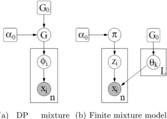
(a) DP mixture model
(b) Finite mixture model
Figure. 2Graphical model
3.1 Dirichlet process
DP is one of the most popular prior used in the Bayesian non-parametric model. Its first use by the machine learning community dates back to [35, 36]. In general, a stochastic process is a probability distribution over a space of paths which describe the evolution of some random value over time. DP is a family of stochastic processes whose paths are probability distributions. It can be seen as an infinite-dimensional generalization of Dirichlet distribution, where it is a prior over the space of countably infinite distributions. In the literature, DP has been constructed in different ways, the most well-known constructions are: infinite mixture model [36], distribution over distributions [37], Polya-urn scheme [38] and stick-breaking [34]. For more details, the interested reader is referred to [39].
Figure 2 shows two graphical models, DP mixture model and the finite mixture model with number of clustersLwhich becomes an infinite mixture model whenLgoes to∞. Infinite mixture model is simply a generalization of the finite mixture model, where DP prior with infinite param-eters is used instead of Dirichlet distribution prior with fixed number of paramparam-eters. The finite mixture model can be represented by the following equations:
π|α0∼Dirichlet(α0/L, ..., α0/L) zi|π∼Discrete(π1, ..., πL) θk|G0∼G0
xi|zi,θ∼F(θzi) (16)
F(θzi) denotes the distribution of the observationxigivenθz i, whereθz iis the parameter vector
associated with componentzi. Herezi indicates which latent cluster is associated with observation xi. Indicatorziis drawn from a discrete distribution governed by parameterπdrawn from dirichlet distribution parametrized byα0. We can simply say thatxi is distributed according to a mixture of components drawn from prior distributionG0 and picked with probability given by the vector of mixing proportionsπ. The model represented by Eq.(16) above is a finite mixture model, where Lis the fixed number of parameters (components). The infinite mixture model can be derived by lettingL→ ∞, then π can be represented as an infinite mixing proportion distributed according to stick-breaking processGEM(α) [34]. Thus, Eq.(16) can be equivalently expressed according to the graphical representation as:
G|α, G0∼DP(α, G0) θi|G∼G
xi|θi∼F(θi) (17)
whereG=P∞
k=1πkδθi is drawn from DP prior,δθi is a Dirac delta function centred atθi.
Tech-nically, DP is a distribution over distribution [37], whereDP(G0, α), is parametrized by the base distributionG0, and the concentration parameterα. Since DP is distribution over distributions, a
Figure. 3Infinite mixture model
drawG from it is a distribution. Thus, we can sample θi from G. Back to Eq.(16), by integrat-ing over the mixintegrat-ing proportion π, we can write the prior for zi as conditional probability of the following form [40]: p(zi=c|z1, ..., zi−1) = n−i c +α0/L i−1 +α0 (18) wheren−i
c is the number ofziforj < ithat are equal toc. By lettingLgoes to infinity we get the following equations: P(zi=c|z1, ..., zi−1)→ n−i c i−1 +α0 P(zi6=zjf or all j < i|z1, ..., zi−1)→ α0 i−1 +α0 (19) For an observation xi with zi 6= zjf or all j < i, a new component gets created with indicator zi=cnew. For more details about the process of obtaining the prior distribution, reader is referred to [40].
3.2 Proposed Model
For the sake of simplification, we start with an unsupervised clustering model, then we add a new ingredient to the model in order to accommodate labelled data.
Unsupervised clustering Figure 3 shows the infinite mixture model whereπ is drawn from a stick-breaking processGEM(α) andG0is a Normal-Inverse-Wishart distributionN IW(.|µ0,Σ0, k0, v0). Whereµ0is the prior of the clusters’ means,Σ0controls the variance among their means,k0scales the diffusion of the clusters means andv0 is the degree of freedom of the Inverse-Wishart distribu-tion. Given the concentration parameterα0and the prior distribution parameters{µ0,Σ0, k0, v0}, we aim at computing online the probability of the current data assignment to the existing clusters p(zt|xt,x1:t−1) without the need for saving all datax1:t−1.
p(zt|xt,x1:t−1) = X z1:t−1 p(zt|z1:t−1,xt,x1:t−1)p(z1:t−1|xt,x1:t−1) p(zt|z1:t−1,xt,x1:t−1)∝p(xt|zt, z1:t−1,x1:t−1)p(zt|z1:t−1) p(z1:t−1|xt,x1:t−1)∝p(xt|z1:t−1,x1:t−1)p(z1:t−1|x1:t−1) (20)
Following [27], we define a state vectorHtthat summarizes the data seen up to timet.Ht=
{zt, mt,nt,st}wheremt is the number of components,ntis the number of data assigned to each component and st is the sufficient statistics for each mixture component. The data x1:t−1 along with their assignmentsz1:t−1 in the first term of the second Equ. in (20) can be replaced byHt−1:
p(xt|zt, z1:t−1,x1:t−1) =p(xt|zt, Ht−1) =
Z
θ
Ifzt refers to a new component,p(θ|zt, Ht−1) becomes equivalent to the prior G0. Otherwise,zt refers to an already existing component. Then p(θ|zt, Ht−1) becomes equivalent to p(θ|szt,t−1). The sufficient statistics (mean, covariance)szt,t−1={suzt,t−1,sczt,t−1}, where
suzt,t−1= P zi=zt,i<txi nzt,t−1 sczt,t−1= X zi=zt,i<t (xi−suzt,t−1)(xi−suzt,t−1)T (22)
Thus, Eq.21 can be solved givenHt−1 and G0. More details can be found in the Appendix. The first term of the third Equation in (20) can be written as follows:
p(xt|z1:t−1,x1:t−1) =
X
zt
p(xt|zt, z1:t−1,x1:t−1)p(zt|z1:t−1) (23)
The assignmentz1:t−1 in the rest of Eq.(20) can be replaced byHt−1.
p(zt|z1:t−1) =p(zt|Ht−1) (24)
p(z1:t−1|x1:t−1) =p(Ht−1|x1:t−1) (25)
Equation (24) has the same solution as Eq.(19). Equation (25) is the posterior of the state vector Ht−1which must be inferred online. Thus, the task is to track the posterior ofHtonline. Assume that the posterior p(Ht−1|x1:t−1) is known, we need to find the updated posterior p(Ht|x1:t). As the number of assignments configurations grows exponentially, it is impossible to compute the distribution over all possibleHt−1. To solve this problem, we resort to particle filters to approximate the posterior by a set ofN weighted particles.
p(Ht|x1:t) = N X i=1 w(i)t δ(Ht−H (i) t ) (26)
where eachHt(i) represents the state vector with different assignmentsz1:tof the data seen so far. The weightwt(i)reflects the importance of the particle andδis the dirac delta function. So, given a set ofN particles and their normalized weights at timet−1, we can approximate the posterior at timetin two steps:
Updating:
p(Ht|x1:t)∝
Z
Ht−1
p(Ht|Ht−1,xt)p(xt|Ht−1)p(Ht−1|x1:t−1) (27)
Given a particleHt(i)−1along with its weightw(i)t−1, the update can be written as follow.
p(Ht|x1:t)∝ N X i=1 p(Ht|H (i) t−1,xt)p(xt|H (i) t−1)w (i) t−1 (28)
Following the update step, the number of resulting particles for eachHt(i)−1 equals to the number of existing componentsm(i)t−1+ 1. The new assignmentsztexpresses the different configurations of the new particles. Therefore,
p(Ht(j)|Ht(i)−1,xt) =p(zt=j|H (i) t−1,xt) ∝p(xt|zt=j, H (i) t−1)p(zt=j|H (i) t−1) (29)
Equation (29) can be solved in the same way as we did in Eq. (21) and (24). The elements of new state vectorHt(j)are updated as folows
Htj = zt =j j is an old component nj,t =λnj,t−1+ 1 nk,t =λnk,t−1 ∀k6=j, k≤mt suj,t = λnj,t−1suj,t−1+xt nj,t scj,t =λscj,t−1+nj,t−1suj,t−1suTj,t−1 −nj,tsuj,tsuTj,t+xtxTt zt =mt−1+ 1 j is a new component mt =mt−1+ 1 nj,t = 1 nk,t =λnk,t−1 ∀k≤mt−1 suj,t =xt scj,t =0 (30)
The second term of Eq.(28) can be written as follows p(xt|H (i) t−1) = X zt p(xt|zt, H (i) t−1)p(zt|H (i) t−1) (31)
whereλis a forgetting factor which allows the components to adapt with change. Equation (31) can be solved in the same way as Eq.(29). Having approximated all the terms of Eq.(28), we end up withM =PN
i=1(m i
t−1+ 1) new particles along with their weightw j
t. So, we move to the next step which reduces the number of created particles to a fix numberN.
Re-sampling:
We follow the resampling technique proposed in [28] which discourages the less-likely particles (configurations) and improves the particles that explain the data better. It keeps the particles whose weight is greater than 1/c, and re-samples from the remaining particles. The variable c is the solution of the following equation:
M
X
j=1
min{cwtj,1}=N (32)
The weight of re-sampled particles is set to 1/cand the weight of the particles greater than 1/cis kept unchanged.
Next, we consider the labels by proposing stick-breaking prior over the classes.
Semi-supervised clustering The stick-breaking component assignment is the same as the Gaus-sian component assignment. That is, every GausGaus-sian component is associated with a stick-breaking oneGEM(α1) and the variablezt controls the component selection (see Fig.4).
Assume that at timet, we need to predict the distribution overytgiven all the data and their labels seen so far.
p(yt|xt, Dt−1) =
X
zt
p(yt|zt, Dt−1)p(zt|Dt−1,xt) (33)
The first term of Eq.(33) can be computed in a similar way as Eq.(19), whereztselects the stick-breaking component generatingyt. Hence, the probability ofytdepends only on the data assigned to componentzt. More details can be found in the appendix
p(yt|zt, Dt−1)∝ ( n0z t,yt,t yt is an existing class α1 yt is a new class (34)
wheren0zt,yt,trefers to the number of the data which are assigned to componentztand have labelyt at timet. So, to compute (34), the distribution of the labels to the data in each component must be
Figure. 4Proposed semi-supervised clustering model
memorized. The second term of Eq.(33) is similar to (20) but with additional observationy1:t−1. We
propose to include the label information in the state vectorHtso that it becomesHt0={Ht,n0t}, wheren0tis the label distribution over the data in each component. Hence,p(zt|Dt−1,xt) is solved in the same way as in Eq.(19) after replacingHt−1 byHt0−1. Similar to what we did in Eq.(25), the posterior of the state vectorHt0−1must be tracked online. Similar to the previous unsupervised model, we resort to particle filters to approximate the posterior by a set ofN weighted particles.
p(Ht0|Dt) = N
X
i=1
w0t(i)δ(Ht0−Ht0(i)) (35)
We can approximate the posterior at time t using two steps; updating and sampling. The re-sampling step is the same as in the unsupervised clustering; we just replace the old weights with the new ones. The updating step follows the same way as in the unsupervised clustering.
p(Ht0|Dt)∝ N X i=1 p(Ht0|Ht0(i)−1,xt, yt)p(xt, yt|H 0(i) t−1)w 0(i) t−1 (36) p(Ht0(j)|Ht0(i)−1,xt, yt) =p(zt=j|H0 (i) t−1,xt, yt)∝ p(xt, yt|zt=j, H0 (i) t−1)p(zt=j|H0 (i) t−1) (37) p(xt, yt|zt=j, H 0(i) t−1) =p(xt|zt=j, H 0(i) t−1)p(yt|zt=j, H 0(i) t−1)) (38)
The second term of Eq.(37) is computed in Eq.(24). Equation (38) can be solved in the same way as the first term in Eq.(33) and Eq.(34). The elements of the new state vector are updated in the same way as in Eq.(30):
Ht0j= n0j,y t,t=λ 0n0
j,yt,t−1+ 1 j is an old component n0k,t=λ0n0k,t−1 ∀k6=j, k≤mt Htj n0j,y t,t= 1 j is a new component n0k,t=λ0n0k,t−1 ∀k6=j, k≤mt Htj (39) p(xt, yt|H 0(i) t−1) = X zt p(xt, yt|zt, H 0(i) t−1)p(zt|H 0(i) t−1) (40)
The estimation ofp(yt+1|xt+1, Dt)) in SAL is computed in Eq.(33). p(xt|x1:t−1) =
X
z1:t−1
p(xt|z1:t−1,x1:t−1)p(z1:t−1|x1:t−1) (41)
where the terms of Eq.(41) are computed as in Eq.(20). The estimation of p(xt|xUt−1) and
Table. 1Benchmark Datasets propreties used for comparing against [33] Datasets N d NcS% L%
Pageblocks 5473 10 5 0.49 89.28 Forest 10000 55 7 12.6 16.2 KDD 23535 41 10 0.042 83.47
Table. 2Benchmark datasets following [43, 44] Datasets N d NcS% L%
Pageblocks 5473 10 5 0.49 89.28 Forest 5000 10 7 3.56 24.36 KDD 33650 41 15 0.04 51.46
the unlabelled dataHu
t and one for the labelled dataHtl. To sum up, three estimator model repre-sented by state vectors associated with their weights:{(Ht0, w0t), (Hu
t, wut) and (Htl, wtl)} and their hyper-parameters:{(α0, α1,µ0,Σ0, k0, v0), (αu0, αu1,µu0,Σ u 0, ku0, vu0) and (α0l, αl1,µl0,Σ l 0, k0l, v0l)}are maintained.
4
Experiments
We evaluate SAL on three real-world benchmark datasets widely used in the AL area: Page-blocks, Covertype (Forest) and KDDCup 99 network intrusion detection (KDD). These datasets are downloaded from UCI repository [41]. SAL is compared against two types of stream-based AL approaches. The first type of approaches [33] does consider challenges of data stream namely theinfinite length of the data andconcept drift, but ignoreconcept evolution. The methods based on [33] are as follows:
- VarUn: Variable Uncertainty, stream-based AL.
- RanVarUn: Variable Randomized Uncertainty, stream-based AL.
We also consider A baseline random sampling:Rand. The aim of this comparison is to show how SAL performs against these methods just cited (with restricted budget). Fortunately, these methods are integrated in the MOA data stream software suite [42] which helps carry out the experiments without the need to implementing them.
The second type of stream-based AL approaches are developed to cope with concept evolu-tion [43, 44]. However, they do not explicitly handle concept drift and avoid the sampling bias problem. More details about these methods are discussed in Sec.??. We consider the following
- lowlik: Low-likelihood criterion specialized for quick unknown class discovery [44] - qbc: Query-by-Commitee, a stream-based verion is used in [43]
- qbc-pyp: Stream-based joint exploration-explotation AL proposed in [44]
These methods have shown good class discovery performance on unbalanced data including the datasets that we use in this study. Hence, by comparing against them, we highlight the efficiency of SAL in handling theconcept evolutionin challenging setting where the class of the datasets are highly unbalanced. We set up the same settings described in [43].
For all the experiments, the number of particles N is set to 5. Normally, as we increase the number of particles, the estimator model gives better estimation, but the computation becomes heavier.
All experiments are repeated 30 times and the results are averaged in order to capture the real performance of SAL.
4.1 datasets
The three datasets Pageblocks, Forest and KDD show multiple classes in naturally unbalanced proportions. Such property will help manifest the capability of SAL to efficiently discover the unknown classes while querying data samples that result in good classification performance. The datasets are presented in Tab.1 and Tab.2, where where N is the number of instances, dis the
Table. 3SAL hyper-parameters setting for comparing against [33] Hyper-parametersα0 αu0 αl0 µ0 µu0 µl0 Σ0 Σ0uΣ0l Values 1 0 Eq. (42) Hyper-parametersv0v0uv l 0 α1k0ku0 k l 0 Values d+ 2 0.01
number of features/attributes,Ncis the number of classes,S% andL% are proportions of smallest and largest classes, respectively.
Pageblocks dataset: the task is to separate text from graphic area of the page layout docu-ment. Thus, the classifier has to classify the blocks of the page detected by a segmentation process. The blocks classes are text, horizontal line, picture, vertical line and graphic.
Forest dataset: this dataset is often used as a benchmark for evaluating stream classifiers. The task is to predict forest cover type from cartographic variables.
KDD dataset: This dataset contains TCP connection records extracted from LAN network traffic at MIT Lincoln Labs over a period of two weeks. Each record refers either to a normal connection or attack.
In this paper, we use the full Pageblocks but only portions of Forest and KDD datasets. When comparing against the first type of competitors [33], We use 10000 instances from the forest dataset and 23535 instances from KDD dataset. As for the second type of competitors [43, 44], we follows the setting in [43] where 5000 and 33650 instances are used from Forest and KDD respectively.
4.2 Classification performance
In this section, we evaluate SAL against the methods in [33] in order to study classification effi-ciency.
Settings As we have shown previously, SAL is flexible and any learner (classifier) can be simply plugged in. Here, we use Naive Bayes as a learner as in [33].
The evaluation of the algorithms is based on a prequential methodology: each time we get an instance, first we compute the probability of querying it. If selected, then it is used to train the learner (classifier). Otherwise, it is used for testing the classifier given that all samples labels are known insight. The classification performance of SAL is measured according to the average accuracy which is the correctly classified data samples divide by the total testing data samples.
The hyper-parameters of the estimator model are fixed apriori (see Tab. 3). However, changing their values has slight effect on the final results. In order to allow obscure prior, we setα0, α0u andαl
0 to 1. The meansu0, uu0 and ul0 are set to 0. The covariance matrices Σ0,Σ0u and Σ0l are roughly set to be as large as the dispersion of the data. We set them to the identity matrix times the distance between the two farest points in the data:
max (x1,x2)∈X
(||x1x2||)I (42)
The degree of freedom of the Wishart distributions v0, vu0 , vl0 must be greater than d. We set them to d+ 2. The hyper-parameters k0, k0u and k0l are empirically set to 0.01. Because at this stage, we are interested only in the classification error, the hyper-parameterα1which controls the prior over the classes is set to a low value. It can be seen from Eq. (34) that whenα1 is low the model tends to put low probability on the emergence of new classes. We empirically set it to 0.01. The effect of the forgetting factorsλandλ0 in Eq.(30) and Eq.(39) on SAL classification accuracy is studied in Fig. 6, Fig.7 and Fig8. We, first, set the forgetting factorsλ0 to 0.6 and study the effect ofλfor the three datasets. Then, we setλto the values that result in the best accuracy and study the effect ofλ0. Finally, the forgetting factors λ andλ0 are set to the values that result in the best accuracy. However, we can notice that the accuracy is almost insensitive to the change of the forgetting factors values.
The proposed non-parametric Bayesian model tackles the lack of prior knowledge about the streaming data where the parameter settings of SAL estimator model are almost the same for all the three datasets. SAL performance is almost insensitive to the parameter settings of the model.
(a) Pageblocks dataset (b) Forest dataset
(c) KDD dataset
Figure. 5 Classification performance
Performance Analysis Following similar setting in [33], we carry out the experiments on the three datasets using different budget values [0.01; 0.4]. Figure 5 shows the classification accuracy of SAL and the competitors for diffrent values of budgetBd.
SAL noticeably outperforms the competitors on the three datasets. While the competitors show inconsistency especially on Pageblock dataset, SAL provides classification accuracy which consistently increases as more data samples are queried. For example, VarUn and RanVarUnc produce fluctuating accuracy on Pageblocks dataset for Bd = 0.05, 0.1, 0.2, 0.25, 0.3, 0.35 and 0.4. Moreover, the baseline Rand outperforms VarUn and RanVarUnc for some budget values. When using the Forest dataset,Rand shows comparable performance toVarUn andRanVarUnc. As for KDD dataset, even though the accuracy almost converges when using budget over 0.3, SAL strongly beats Rand,VarUn and RanVarUnc using budget less than 0.1. Such superior accuracy with low budget is a very strong point for SAL as it aligns with the goal of AL which is high accuracy with low budget.
The reasons why SAL outperforms the competitors are rooted from the fact that SAL tries to directly minimize the expected future error instead of employing heuristic AL criteria as the competitors do. We can intuitively highlight two main differences between SAL and the competitors AL approaches. Firstly, SAL explicitly handles sampling bias problem resulting in drift aware AL strategy. On the other side,RanVarUn combines naive randomization with stationary online uncertainty criterion to deal with drift. By doing so, the budget is wasted on some random queries. VarUncdoes not handlesampling bias problem. Secondly, SAL takes into account the importance of data marginal distribution while the competitors do not.
Table. 4Number of classes discovered by different methods Datasets Nclowlik qbc qbc−pyp SAL
Pageblocks 5 4.72 3.42 5 5
Forest 7 7 7 7 7
KDD 15 9.76 3.32 8.71 8
Table. 5Average class accuracy achieved using different methods Datasets lowlik qbc qbc−pyp SAL
Pageblocks 63.23 45.79 71.72 65.65 Forest 57.13 58.68 58.45 58.71 KDD 51.21 19.42 47.35 45.14
4.3 Class discovery performance
In order to highlight the capability ofconcept evolution(class discovery), SAL is compared against [43, 44], the state-of-the-art methods.
Settings The performance of SAL is measured using the average class accuracy [45]. The final accuracy is obtained by averaging accuracies. It is worth mentioning that the final class accuracy is fairly penalized when there are mi-classifications in small classes.
SAL takes into account the data density when querying. It might then consider the data repre-senting small classes as outliers or noise and therefore never queries them. To avoid such a scenario and to improve the class discovery performance of SAL, we increase the importance of the small classes by integrating online their effect in the loss functionL(.). In other words, we weight the loss according to the size of the classes seen at timet. Thus, the loss in Eq.(10) and Eq.(11) is formulated as follows:
L0(ˆp(y|x), p(y|x)) = 1
s(y)L(ˆp(y|x), p(y|x)) (43) wheres(y) represents the importance of the class. It is proportional to the number of samples from a classy. To consider the dynamic nature of the data, we use a forgetting factor instead of counting all the samples seen so far. If the class is new, the weight is equal to one. All the parameters of the estimator model excludingα1 are set to the same values as in the previous section. Because α1 controls the prior over the classes, therefore, it has impact on the class discovery performance. As shown in Eq.(34), the model tends to put high probability on the emergence of new classes whenα1is high. We studied its effect on each dataset. So, it is set to 0.5 for Pageblocks and KDD and 0.4 for Forest. We can see that the value ofα1 for Forest dataset is less than the others. Such difference can be interpreted as a result of the less unbalance classes in the Forset dataset compared to Pageblocks and KDD datasets.
Performance AnalysisIn these experiments, we follow the same setting as in the competitors [43, 44], where the maximun number of queries is set to 150 instances (SAL takes the budget ratio as input).
The results of the experiments are shown in Tab.4 and Tab.5. Table 4 presents the number of classes discovered by the different methods. Table 5 presents the average class accuracy achieved using the different methods. The results show that SAL provides a comparable class discovery performance compared to the competitors. SAL was able to discover all the classes for the Page-blocks and Forest datasets and 8 out of 15 classes for the KDD data (see Tab.4). Its average class accuracy is the best on the Forest data which can be explained by the fact that the data is less unbalanced. That might be a result of SAL consideration of the data density which has shown good classification performance in the previous section. As for Pageblocks and KDD, SAL has the second and third best results among the competitors.
4.4 Discussion
While SAL shows far better classification performance than all the competitors on all datasets, its class discovery performance is not the best on all of them. The reason can be rooted to SAL outliers
avoidance. This latter along with the sampling bias mechanism have led to strong classification performance. Nonetheless, the class discovery performance is comparable to strong competitors which some of them are specialized for detecting the outliers as novel classes. Furthermore, SAL has shown better class discovery performance on the Forest data which class unbalance is less sever. To conclude, SAL can be reliably used for novelty detection tasks, however, there might be better alternative. On the other hand, SAL is a strong method for task requiring high classification performance where the number of classes is unknown. In this latter, the focus is on the classification performance, where the error for all data samples are the same and no penalization is applied or the emergent classes are mostly normal.
5
Conclusion and future work
We proposed an active learning algorithm for data streams capable of dealing with data streams challenges:infinite length,concept drift andconcept evolution. The SAL algorithm labels the sam-ples that reduce the future expected error in a completely online scenario. It also tackles the sampling bias of active learning. Experimental results on real-world data showed the limitation of the proposed approach regarding class discovery when applying to highly unbalanced datasets. However, the main goal of the proposed algorithm is to perform classification with unknown num-ber of classes. Furthermore, its class discovery performance is comparable to the state-of-the-art and sometime better when the classes are not severely unbalanced.
In future investigations, we will employ the proposed method on a real world application e.g, AR is a strong candidate. However, in such scenarios we might need to consider more challenges such as the labelling delay.
Acknowledgment
A. Bouchachia was supported by the European Commission under the Horizon 2020 Grant 687691 related to the project:PROTEUS: Scalable Online Machine Learning for Predictive Analytics and Real-Time Interactive Visualization.
References
1. G. Hulten, L. Spencer, and P. Domingos, “Mining time-changing data streams,” inProceedings of the seventh ACM SIGKDD international conference on Knowledge discovery and data mining. ACM, 2001, pp. 97–106.
2. Y. Yang, X. Wu, and X. Zhu, “Combining proactive and reactive predictions for data streams,” in
Proceedings of the eleventh ACM SIGKDD international conference on Knowledge discovery in data mining. ACM, 2005, pp. 710–715.
3. C. C. Aggarwal, Data streams: models and algorithms. Springer Science & Business Media, 2007, vol. 31.
4. M. M. Gaber, A. Zaslavsky, and S. Krishnaswamy, “Mining data streams: a review,” ACM Sigmod Record, vol. 34, no. 2, pp. 18–26, 2005.
5. P. Domingos and G. Hulten, “Mining high-speed data streams,” in Proceedings of the sixth ACM SIGKDD international conference on Knowledge discovery and data mining. ACM, 2000, pp. 71–80. 6. M. Sayed-Mouchaweh,Learning from Data Streams in Dynamic Environments. Springer, 2016. 7. J. Gama, I. ˇZliobait˙e, A. Bifet, M. Pechenizkiy, and A. Bouchachia, “A survey on concept drift
adap-tation,”ACM Computing Surveys (CSUR), vol. 46, no. 4, p. 44, 2014.
8. M. Sayed-Mouchaweh, “Handling concept drift,” inLearning from Data Streams in Dynamic Environ-ments. Springer, 2016, pp. 33–59.
9. A. Bouchachia and C. Vanaret, “Gt2fc: an online growing interval type-2 self-learning fuzzy classifier,”
Fuzzy Systems, IEEE Transactions on, vol. 22, no. 4, pp. 999–1018, 2014.
10. C. C. Aggarwal, J. Han, J. Wang, and P. S. Yu, “A framework for on-demand classification of evolving data streams,”Knowledge and Data Engineering, IEEE Transactions on, vol. 18, no. 5, pp. 577–589, 2006.
11. A. Bouchachia, “Incremental learning with multi-level adaptation,”Neurocomputing, vol. 74, no. 11, pp. 1785–1799, 2011.
12. Y. Sun, K. Tang, L. L. Minku, S. Wang, and X. Yao, “Online ensemble learning of data streams with gradually evolved classes,”IEEE Transactions on Knowledge and Data Engineering, vol. 28, no. 6, pp. 1532–1545, 2016.
13. M. M. Masud, Q. Chen, L. Khan, C. Aggarwal, J. Gao, J. Han, and B. Thuraisingham, “Address-ing concept-evolution in concept-drift“Address-ing data streams,” in Data Mining (ICDM), 2010 IEEE 10th International Conference on. IEEE, 2010, pp. 929–934.
14. M. M. Masud, J. Gao, L. Khan, J. Han, and B. Thuraisingham, “Classification and novel class detection in concept-drifting data streams under time constraints,” Knowledge and Data Engineering, IEEE Transactions on, vol. 23, no. 6, pp. 859–874, 2011.
15. T. Al-Khateeb, M. M. Masud, L. Khan, C. Aggarwal, J. Han, and B. Thuraisingham, “Stream classifi-cation with recurring and novel class detection using class-based ensemble,” inData Mining (ICDM), 2012 IEEE 12th International Conference on. IEEE, 2012, pp. 31–40.
16. M. A. Pimentel, D. A. Clifton, L. Clifton, and L. Tarassenko, “A review of novelty detection,”Signal Processing, vol. 99, pp. 215–249, 2014.
17. R. P. Adams and D. J. MacKay, “Bayesian online changepoint detection,” arXiv preprint arXiv:0710.3742, 2007.
18. S. Dasgupta, “Two faces of active learning,”Theoretical computer science, vol. 412, no. 19, pp. 1767– 1781, 2011.
19. D. A. Cohn, Z. Ghahramani, and M. I. Jordan, “Active learning with statistical models,”Journal of artificial intelligence research, 1996.
20. N. Roy and A. McCallum, “Toward optimal active learning through monte carlo estimation of error reduction,”ICML, Williamstown, pp. 441–448, 2001.
21. S. Vijayanarasimhan and K. Grauman, “Multi-level active prediction of useful image annotations for recognition,” inAdvances in Neural Information Processing Systems, 2009, pp. 1705–1712.
22. Mohamad, Bouchachia, and Sayed-Mouchaweh, “A bi-criteria active learning algorithm for dynamic data streams,”IEEE transactions on neural networks and learning systems (Minor revision, 2016). 23. Y. W. Teh, “Dirichlet process,” inEncyclopedia of machine learning. Springer, 2011, pp. 280–287. 24. J. Sethuraman, “A constructive definition of dirichlet priors,”Statistica sinica, pp. 639–650, 1994. 25. P. Del Moral, A. Doucet, and A. Jasra, “Sequential monte carlo samplers,” Journal of the Royal
Statistical Society: Series B (Statistical Methodology), vol. 68, no. 3, pp. 411–436, 2006.
26. O. Capp´e, S. J. Godsill, and E. Moulines, “An overview of existing methods and recent advances in sequential monte carlo,”Proceedings of the IEEE, vol. 95, no. 5, pp. 899–924, 2007.
27. C. M. Carvalho, H. F. Lopes, N. G. Polson, M. A. Taddyet al., “Particle learning for general mixtures,”
Bayesian Analysis, vol. 5, no. 4, pp. 709–740, 2010.
28. P. Fearnhead, “Particle filters for mixture models with an unknown number of components,”Statistics and Computing, vol. 14, no. 1, pp. 11–21, 2004.
29. A. Doucet, N. De Freitas, and N. Gordon, “An introduction to sequential monte carlo methods,” in
Sequential Monte Carlo methods in practice. Springer, 2001, pp. 3–14.
30. Y. ¨Ulker, B. G¨unsel, and A. T. Cemgil, “Sequential monte carlo samplers for dirichlet process mix-tures,” inInternational Conference on Artificial Intelligence and Statistics, 2010, pp. 876–883. 31. W. Chu, M. Zinkevich, L. Li, A. Thomas, and B. Tseng, “Unbiased online active learning in data
streams,” inProceedings of the 17th ACM SIGKDD international conference on Knowledge discovery and data mining. ACM, 2011, pp. 195–203.
32. A. Beygelzimer, S. Dasgupta, and J. Langford, “Importance weighted active learning,” inProceedings of the 26th Annual International Conference on Machine Learning. ACM, 2009, pp. 49–56.
33. I. Zliobaite, A. Bifet, B. Pfahringer, and G. Holmes, “Active learning with drifting streaming data,”
Neural Networks and Learning Systems, IEEE Transactions on, vol. 25, no. 1, pp. 27–39, 2014. 34. J. Sethuraman, “A constructive definition of dirichlet priors,” DTIC Document, Tech. Rep., 1991. 35. R. M. Neal, “Bayesian mixture modeling,” inMaximum Entropy and Bayesian Methods. Springer,
1992, pp. 197–211.
36. C. E. Rasmussen, “The infinite gaussian mixture model.” inNIPS, vol. 12, 1999, pp. 554–560. 37. T. S. Ferguson, “A bayesian analysis of some nonparametric problems,”The annals of statistics, pp.
209–230, 1973.
38. D. Blackwell and J. B. MacQueen, “Ferguson distributions via p´olya urn schemes,” The annals of statistics, pp. 353–355, 1973.
39. Y. W. Teh, “Dirichlet process,” inEncyclopedia of machine learning. Springer, 2010, pp. 280–287. 40. R. M. Neal, “Markov chain sampling methods for dirichlet process mixture models,”Journal of
com-putational and graphical statistics, vol. 9, no. 2, pp. 249–265, 2000. 41. A. Asuncion and D. Newman, “Uci machine learning repository,” 2007.
42. A. Bifet, G. Holmes, R. Kirkby, and B. Pfahringer, “Moa: Massive online analysis,”Journal of Machine Learning Research, vol. 11, no. May, pp. 1601–1604, 2010.
43. C. C. Loy, T. M. Hospedales, T. Xiang, and S. Gong, “Stream-based joint exploration-exploitation active learning,” in Computer Vision and Pattern Recognition (CVPR), 2012 IEEE Conference on. IEEE, 2012, pp. 1560–1567.
44. C. C. Loy, T. Xiang, and S. Gong, “Stream-based active unusual event detection,” inAsian Conference on Computer Vision. Springer, 2010, pp. 161–175.
45. T. M. Hospedales, S. Gong, and T. Xiang, “Finding rare classes: Active learning with generative and discriminative models,”IEEE transactions on knowledge and data engineering, vol. 25, no. 2, pp. 374–386, 2013.
Appendix
Compute Equ. (21): p(xt|zt, z1:t−1,x1:t−1) =p(xt|zt, Ht−1) = Z θ p(xt|θ)p(θ|zt, Ht−1) (44)– Ifztrefers to a new component: p(xt|zt, Ht−1) =
Z
θ
p(xt|θ)p(θ|G0) =tv1(xt|µ1,Σ1) (45)
wheretrefer to student’s t-distribution which we end up with as a result of using a conjugate prior (i.e., the Normal Inverse Wishart prior) over the normal distribution parameterθ.
µ1=µ0 (46) Σ1= Σ0(k0+ 1) k0(v0−d+ 1) (47) v1=v0−d+ 1 (48)
wheredis the dimension of the data.
– Ifztrefers to an already seen component: p(xt|zt, Ht−1) = Z θ p(xt|θ)p(θ|szt,t−1, nzt,t−1) =tv2(xt|µ2,Σ2) (49) µ2= k0 k0+nzt,t−1 µ0+ nzt,t−1 k0+nzt,t−1 suzt,t−1 (50) Σ2= 1 (k0+nzt,t−1)(v0+nzt,t−1−d+ 1) Σ0+sczt,t−1+ k0nzt,t−1 k0+nzt,t−1 (suzt,t−1−µ0)(suzt,t−1−µ0) T (k0+nzt,t−1+ 1) (51) v2=v0+nzt,t−1−d+ 1 (52)
Compute the first term of Equ. (33):
Givenzt, ytis independent of the observationsx1:t−1. Hence,
p(yt|zt, Dt−1) =p(yt|zt, yt−1) (53)
Aszt selects the stick breaking component generating yt, the distribution ofyt depends only on the label of the data assigned to components zt. By marginalizing the selected stick breaking component the same way as in Eq.(19), we end up with the following equations:
p(yt|zt, Dt−1) = nzt,yt,t α1+n0zt,t−1 ∝n 0
zt,yt,t ytis an existing class α1
α1+n0zt,t−1 ∝α1 ytis a new class
(a) Forgetting factorsλ (b) Forgetting factorsλ0
Figure. 6Pageblocks data (budget 0.03)
(a) Forgetting factorsλ (b) Forgetting factorsλ0
Figure. 7Forest data (budget 0.1)
(a) Forgetting factorsλ (b) Forgetting factorsλ0