DOI 10.1007/s10994-012-5279-6
Scalable and efficient multi-label classification
for evolving data streams
Jesse Read·Albert Bifet·Geoff Holmes· Bernhard Pfahringer
Received: 19 October 2010 / Accepted: 20 January 2012 / Published online: 21 February 2012 © The Author(s) 2012
Abstract Many challenging real world problems involve multi-label data streams. Efficient methods exist for multi-label classification in non-streaming scenarios. However, learning in evolving streaming scenarios is more challenging, as classifiers must be able to deal with huge numbers of examples and to adapt to change using limited time and memory while being ready to predict at any point.
This paper proposes a new experimental framework for learning and evaluating on multi-label data streams, and uses it to study the performance of various methods. From this study, we develop a multi-label Hoeffding tree with multi-label classifiers at the leaves. We show empirically that this method is well suited to this challenging task. Using our new frame-work, which allows us to generate realistic multi-label data streams with concept drift (as well as real data), we compare with a selection of baseline methods, as well as new learn-ing methods from the literature, and show that our Hoeffdlearn-ing tree method achieves fast and more accurate performance.
Keywords Multi-label classification·Data streams classification
Editors: Grigorios Tsoumakas, Min-Ling Zhang, and Zhi-Hua Zhou. J. Read currently at: Universidad Carlos III, Spain: E-mail: [email protected].
A. Bifet currently at: Yahoo! Research Barcelona, Catalonia: E-mail: [email protected]. J. Read·A. Bifet (
)·G. Holmes·B. PfahringerComputer Science Department, University of Waikato, Hamilton, New Zealand e-mail:[email protected] J. Read e-mail:[email protected] G. Holmes e-mail:[email protected] B. Pfahringer e-mail:[email protected]
1 Introduction
The trend to larger data sources is clear, both in the real world and the academic literature. Nowadays, data is generated at an ever increasing rate from sensor applications, measure-ments in network monitoring and traffic management, log records or click-streams in web exploration, manufacturing processes, call-detail records, email, blogs, RSS feeds, social networks, and other sources. Real-time analysis of these data streams is becoming a key area of data mining research as the number of applications demanding such processing in-creases.
A data stream environment has different requirements from the traditional batch learning setting. The most significant are the following, as outlined in Bifet and Gavaldà (2009): – process an example at a time, and inspect it only once (at most);
– be ready to predict at any point; – data may be evolving over time; and
– expect an infinite stream, but process it under finite resources (time and memory). In this work we specifically look at the task of multi-label classification; the generalisa-tion of the tradigeneralisa-tional multi-class (single-label) task. In multi-label classificageneralisa-tion, instead of a single class-label, each example can be associated with multiple labels. Multi-label clas-sification has seen considerable development in recent years, but so far most of this work has been carried out in the static context of batch learning where train-then-test scenarios or cross-fold validation evaluations are typical. Despite the fact that most of the example data stream applications above can be applied to multi-label contexts, very few authors have looked explicitly at the task in a data stream context. It is not yet known how well various multi-label approaches function in such a context, and there are no benchmarks to compare to.
The first truly instance-incremental learning approach in a multi-label data stream con-text considering concept drift was presented in Read et al. (2010). In this paper, we extend this work. We argue (and later provide empirical evidence to show) that instance-incremental learning approaches are the best approach for learning from data streams due to two main advantages: (1) they learn from each example as it arrives (and thus maintain a relevant learner), and (2) they do not discard information prematurely. Batch-incremental learning approaches often, therefore, fail to learn a complete concept within typical (or even gener-ous) time and memory constraints, as they must phase out models built on earlier batches, as memory fills up. Moreover, they must wait to fill a batch with incoming examples before they can learn from them.
The main contributions of this paper are:
– a study of the application of existing multi-label methods to evolving data streams; – the development of a framework for learning from and evaluating on multi-label data
streams;
– modelling evolving synthetic multi-label data as part of this framework;
– a high-performance instance-incremental adaptive method which resulted from the afore-mentioned study; and
– an empirical demonstration that our method outperforms base-line methods as well as modern methods from the recent literature, thus creating a new set of benchmarks in predictive performance and time complexity.
In Sect. 2 we review related work, and in Sect.5 we discuss how to deal with con-cept drift. In Sect.3we review our multi-label data stream framework. In Sect.4we detail
our method for generating synthetic multi-label streams. In Sect.6we discuss new meth-ods for multi-label data stream classification as well as the adaptation of existing methmeth-ods. Section7details a first comprehensive cross-method comparison. We summarise and draw conclusions in Sect.8.
2 Related work
We will first look at existing multi-label approaches, and then discuss data stream specific applications.
A simple base-line method for multi-label classification is the binary relevance method (BR).BRtransforms a multi-label problem into multiple binary problems, such that binary models can be employed to learn and predict the relevance of each label.BRhas often been overlooked in the literature because it fails to take into account label correlations directly during the classification process (Godbole and Sarawagi 2004; Tsoumakas and Vlahavas 2007; Read et al.2008), although there are several methods that overcome this limitation (e.g. Cheng and Hüllermeier2009; Godbole and Sarawagi2004; Read et al.2009).BRcan be applied directly to data streams by using incremental binary base models.
An alternative paradigm toBRis the label combination or label powerset method (LC). LC transforms a multi-label problem into a single-label (multi-class) problem by treat-ing all label combinations as atomic labels, i.e. each labelset becomes a streat-ingle class-label within a single-label problem. Thus, the set of single class-labels represents all distinct label subsets in the original multi-label representation. Disadvantages ofLCinclude its worst-case computational complexity and tendency to over-fit the training data, although this problem has been largely overcome by newer methods (Tsoumakas and Vlahavas2007; Read et al.2008).
Another multi-label approach is pairwise classification (PW), where binary models are used for every possible pair of labels (Fürnkranz et al.2008).PWperforms well in some contexts, but the complexity in terms of models ((L×(L−1)/2)forLlabels) means that this approach is usually intractable on larger problems.
Note that these are all problem transformation methods, wherein a multi-label problem is transformed into one or more single-label problems, and any off-the-shelf multi-class classifier (or binary classifier in the case ofBRandPW) can be used. These methods are interesting generally due to their flexibility and general applicability. In fact, all methods in the literature use, mention or compare to at least one of them. Therefore, in this paper we will start by considering them as the basic methods to compare to, using them in combination with off-the-shelf incremental classifiers for data streams.
A number of single-label classifiers have also been adapted directly to multi-label clas-sification, most notably decision trees (Clare and King2001),k-nearest neighbor (Zhang and Zhou2007) and boosting (Schapire and Singer2000). We note that most adaptation methods have some connection with problem transformation.
Let us now look at existing data stream classifiers. A simple approach to the data stream problem is to train a batch-learning classifier on batches of new examples that replace clas-sifiers built from earlier batches over time (Widmer and Kubat1996; Qu et al.2009). We call this approach batch-incremental. This procedure can be made to satisfy the above con-straints, and can be used with any existing learning method. A first approach to multi-label data stream classification was reported in Qu et al. (2009). This method is batch-incremental, usingK batches ofSexamples to train meta-BR(MBR); a well-known multi-label method described in Godbole and Sarawagi (2004), where the outputs of oneBRare used in the
attribute space of a secondBR(a form of stacking, employed to take into account label cor-relations). An additional weighting scheme supplements the standardMBRfunctionality. An MBRclassifier is built on every new batch ofSexamples and replaces the oldest classifier. In this scheme the concept is represented by at mostK×Sexamples. We implement and compare toMBRin our experiments, in this batch-incremental way, and show why instance-incremental methods are advantageous for learning in a data stream environment.
A Hoeffding Tree (Domingos and Hulten2000) is an incremental, anytime decision tree induction algorithm that is capable of learning from massive data streams by exploiting the fact that a small sample is often enough to choose an optimal splitting attribute. Using the Hoeffding bound one can show that the output of a Hoeffding Tree is asymptotically nearly identical to that of a non-incremental learner using infinitely many examples.
In Law and Zaniolo (2005) an incremental and adaptive kNN algorithm is presented; in-cremental Naive Bayes has been used in Cesa-Bianchi et al. (2006); and perceptrons can also be used in incremental settings (Crammer and Singer2003). Kirkby (2007) makes improve-ments to Hoeffding trees and introduces the MOA framework1for data stream generation and classification. Bifet et al. (2009) additionally considers concept drift in this framework, and presents several high-performing ensemble methods employing Hoeffding trees. En-semble learning classifiers often have better accuracy and they are easier to scale and par-allelize than single classifier methods. Oza and Russell (2001) developed online versions of bagging and boosting for data streams. They show how the process of sampling bootstrap replicates from training data can be simulated in a data stream context. So far Hoeffding trees and ensemble methods have proved very successful. In Bifet et al. (2009) new state-of-the-art bagging methods were presented: the most applicable,ADWINBagging using a change detector to decide when to discard under-performing ensemble members, is adapted here for use in a multi-label context.
Using Clare and King (2001)’s entropy adaption toC4.5, Hoeffding trees can be made multi-label, although to our knowledge this has not yet been investigated in the literature until now.
Recently, Kong and Yu (2011) presented an instance-incremental scheme for multi-label classification on data streams by employing an ensemble of random trees. This is a simi-lar idea to the one we presented in Read et al. (2010), which also involved ensembles of random (Hoeffding) trees. A main difference is that, to deal with concept drift, they use simple ‘fading functions’ at the nodes of each tree to simply fade out the influence of past data, rather than using a drift-detection mechanism (as we do) to detect the point of change. Thus, their method assumes that relevance deteriorates directly with time. Furthermore, the results of this work do not show much impact: they only show some improvement over batch-incremental MLkNN (a well known but arguably outdated multi-label kNN-based classifier), which is an unusual choice for comparison sincekNN methods are actually suit-able to an instance-incremental context.
Also in recent work, Spyromitros-Xioufis et al. (2011) studied concept drift in multi-label data in a data stream context, and they introduce a sophisticated parameterised windowing mechanism for dealing with it, which they exemplify with an efficient instance-incremental multi-labelkNN method. Like Kong and Yu (2011), this method does not explicitly try and detect drift, but rather just phases out older examples over time, which could be considered as a disadvantage when compared to the methods presented in this paper. However, unlike Kong and Yu (2011) this classification method realises the potential ofkNN as an instance-incremental method, and we compare to it in our experiments.
In a regression context, an arguably similar setting to label learning is the multi-target problem, that is addressed in Appice and Džeroski (2007), and on data streams in Ikonomovska et al. (2011). However, we are not aware of any existing work dealing with this approach on multi-label data streams; the work done in this paper does not deal with any multi-label data sources, and thus is it not of specific relevance to this paper.
3 A framework for multi-label data stream mining We use the following notation.
– X=RAis the input attribute space ofAattributes – x∈Xis an instance; x= [x1, . . . , xA]
– L= {1, . . . , L}is a set ofLpossible labels – y∈ {0,1}Lrepresents a labelset; y= [y
1, . . . , yL]whereyj =1 ⇐⇒ the jth label is relevant (otherwiseyj=0)
– (xi,yi)is an example; instance and associated label relevances – yj(i)is thejth label relevance of theith example;x(i)
a is theath attribute of theith instance – y is the number of relevant labels
– z≡φLC(D)=N1
N
i=1
y refers to label cardinality: the average number of labels for examples 1, . . . , Nin a datasetD
A classifier hmakes a prediction yˆi=h(xi), which is evaluated against yi, then (xi,yi) becomes a new training example.
Typically, a classifier in a real-world incremental context interleaves classification and training, where new examples are classified (i.e. labelled) automatically as they become available, and can be used for training as soon as their label assignments are confirmed or corrected. It may be a human or community of humans doing the checking (often termed a folksonomy), or checking might be automatic. For example, a robot learns multiple actions to complete a task, and each time it attempts the task, it can auto-evaluate its success.
Our complete framework supplies a way to generate different types of evolving multi-label data (Sect.4), as well as a variety of methods for multi-label classification (Sect.6). In this section we present an incremental multi-label evaluation component.
In multi-label classification, we must deal with the extra dimension ofLbinary relevance classifications per example, as opposed to one simple 0/1 classification accuracy measure.
The Hamming-loss metric is a label-based measure, where the binary relevance of each label is evaluated separatelyL×Nbinary evaluations in total for a window ofNexamples:
Hamming-loss= 1 LN N i=1 L j=1 1y(i) j =y (i) j
A similar, increasingly popular measure is the label-based F-measure where theF1score (commonly used in the information-retrieval community) is calculated separately for each label, then averaged. For a window ofNexamples whereF1(v,vˆ)gives theF1score for two binary vectors: F-measure= 1 L L j=1 F1([yj(1), . . . , y (N ) j ],[ ˆy (1) j , . . . ,yˆ (N ) j ])
The 0/1-loss metric (also known as exact match), is an example-based measure that considers an example classified correctly if and only if all label relevances of that example are correct. For a window ofNexamples:
0/1-loss= 1 N N i=1 1yi= ˆyi
These measures contrast well with each other. We also use the subset accuracy metric (defined in Godbole and Sarawagi2004), which is a trade-off between strict label-based and strict example-based measures; a score (∈ [0,1]) is given for each example. For a window ofNexamples: Accuracy= 1 N N i=1 L j=1y (i) j ∧ ˆy (i) j L j=1y (i) j ∨ ˆy (i) j
As a single measure, accuracy works well: algorithms get a score from partially-correct labelset predictions, unlike 0/1-loss, but it is not purely label-based, as is Hamming-loss and the F-measure. All measures, as we have employed them, consider all labels 1, . . . , L, whether or not they appear in the current window. They must be predicted as zeros (true negatives) to be considered correct.
Given a test example, nearly all multi-label algorithms, including all ensemble methods, initially result in a confidence output vector (e.g. posterior probabilities) where the score for each label is∈ [0,1], and require an extra process to bipartition the labelset into relevant and irrelevant labels to yield a multi-label predictionyˆ= {0,1}L. This is typically a threshold function where yˆj =1 iff the score for thisjth label is greater than a thresholdt. The importance of good threshold tuning is explained in Read (2010).
In Read et al. (2010) we adjusted the threshold instance-by-instance by a small amount depending on the predicted vs actual label cardinality. However, Spyromitros-Xioufis et al. (2011) have reported good results with batch-adjustments, which we have since adopted (except using the single-threshold method we reported in Read et al.2011).
Initially we sett=0.5 for the first window ofwexamples (let’s call this windowW0). Subsequently, we use the threshold on windowWi which best approximated the true label cardinality of windowWi−1. For convenience, we use the samewas the evaluation window (see the following).
Finally, we also consider log-loss for evaluation, which analyses confidence outputs di-rectly. This measure is ideal to make sure that results are not purely dependent on a particular threshold-calibration method. On a window ofNexamples:
Log-Loss= 1 N L N i=1 L j=1
min(log-loss(yˆ(i)j , yj(i)),ln(N ))
where:
log-loss(y, y)ˆ = −(ln(y)yˆ +ln(1− ˆy)(1−y))
All measures have been reviewed in Read (2010) and are commonly used in the litera-ture (e.g. Tsoumakas and Katakis2007; Tsoumakas and Vlahavas2007; Read et al.2009; Cheng et al.2010). We use more of the methods for the later, more extensive and important experiments.
There are two basic evaluation procedures for data streams: holdout evaluation and pre-quential evaluation. Standard estimation procedures for small datasets, such as cross vali-dation, do not apply due to the continuous and time-ordered nature of testing examples in streams.
In data stream mining, the most frequently used measure for evaluating predictive accu-racy of a classifier is prequential accuaccu-racy. Gama et al. (2009) propose a forgetting mech-anism for estimating holdout accuracy using prequential accuracy: either a sliding window of sizewwith the most recent observations can be used, or fading factors that weigh obser-vations using a decay factorα. The output of the two mechanisms is very similar, as every window of sizew0can be approximated by some decay factorα0.
TheMOAframework (Bifet et al.2010) (software available athttp://moa.cs.waikato.ac.nz/) provides an environment for implementing algorithms and running experiments in a data stream context. Synthetic data streams can be generated in addition to using real-world data sets, including concept drift, as it is presented in Bifet et al. (2009).
TheMEKAframework (software available athttp://meka.sourceforge.net) includes well-known methods for multi-label learning, which we updated for incremental classification. These methods can be called fromMOAand, likewise, can useMOAclassifiers.
For this work, we extendMOAto multi-label functionality for using real-world datasets, generating synthetic data, and developing new algorithms for classifying this data, although we currently still useMEKA-implementations for many algorithms. The software used for the experiments in this paper is available athttp://meka.sourceforge.net/ml.html.
In the next section we detail our synthetic-data generator, and—in the section thereafter— our novel methods for classification.
4 Generating synthetic multi-label data
Despite the ubiquitous presence of multi-label data streams in the real world (such as the examples listed in the Introduction), assimilating and storing them on a large scale with both labels and time-order intact has so far proved largely impractical. Furthermore, in-depth domain knowledge may be necessary to determine and pinpoint changes to the concepts represented by the data, making drift-analysis difficult. This fact provides strong motivation for generating synthetic data.
There are several existing methods for generating synthetic multi-label data, for example Park and Fürnkranz (2008), Qu et al. (2009), but most are task-specific and not sufficient for general use. Of these, only Qu et al. (2009) introduces concept shift, by changing generation parameters, but is far too simple, involving only two labels, to be considered as a good approximation of real-world data. Overall, prior methods produce data which contains very few attributes and labels, as few as two to three, and are therefore not a generally good real-world approximation, even though they can be useful for analysing or highlighting particular characteristics of certain algorithms. Our framework contributes a general method which can simulate dependencies between labels as found in real data, as well as any number and type of attributes in the attribute space, and their relationships to the label space. Furthermore, it can realistically simulate how these dependencies and relationships evolve over time. 4.1 Generating multi-label data streams
It is acknowledged in the literature that dependencies exist between labels in multi-label data (Cheng et al.2010; Read et al.2008; Tsoumakas and Vlahavas2007; Dembczy´nski et al.
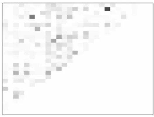
Fig. 1 Pairwise unconditional
dependence on the IMDB dataset, measured with mutual
information: IYj;Yk= yj∈{0,1} yk∈{0,1}p(yj, yk)× logpp(yj,yk) 1(yj)p2(yk). Shades
represent information i.e. dependencies between labels; the
darker the shade the more
information
2010). We can look at these dependencies between labels from a probabilistic point of view, as did Cheng et al. (2010) for classification, where two types of dependency in multi-labelled data were identified: unconditional dependence, a global dependence between labels, and conditional dependence where dependencies are conditioned on a specific instance. The generator method we present is able to incorporate both these types of dependencies in the multi-label data it produces.
4.1.1 Unconditional dependence
Unconditional dependence refers to the idea that certain labels are likely or unlikely to occur together. For example, in the IMDB dataset (see Sect.7.2), labelsRomanceandComedy often occur together, whereasAdultandFamilyare mutually exclusive. Unconditional dependence can be measured with, for example, Pearson’s correlation coefficient or mutual information. Figure1shows pairwise unconditional dependence in the IMDB dataset.
To synthesise unconditional dependence, the following parameters need to be specified: – zthe average number of labels per example (label cardinality);z∈ [0, L]
– uthe ‘amount’ of dependence among the labels;u∈ [0,1]
First we randomly generate a prior probability mass function (pmf)π, whereLj=1πj=
zandπj gives the prior probability of thejth label; i.e.πj:=P (Yj=1).
Fromπ we can generate a conditional distribution:θ over all label pairs. Firstθj k:=
P (Yj=1|Yk=1)for allL≤j > k≤1, whereuof these values are set randomly to be
∈ [min(πj, πk),max(0.0, (πj+πk−1.0))](label dependence) and the rest are set toθj k≈
πj(independence). We then simply apply Bayes rule so thatθkj=(θj k·πk)/πj. Finally, for convenience, we setπto the diagonal ofθ(θjj≡πj) so matrixθis our only parameter. We model label dependence as the joint distribution, calculated as follows, noting that we can get anyP (Yj=yj|Yk=yk)withθusing probability laws:
pθ(y)=p(y1) L j=2
p(yj|yj−1) (1)
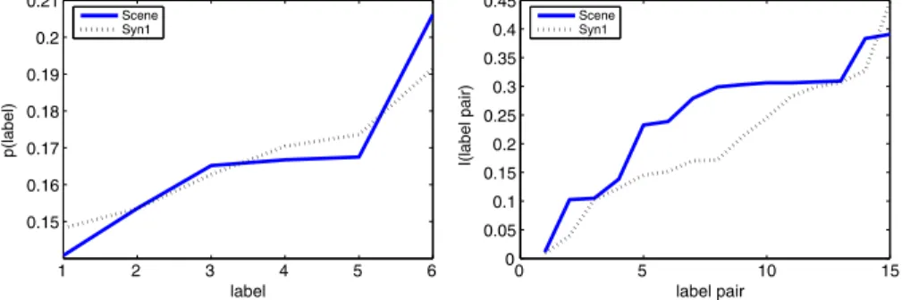
Real-world multi-label data varies considerably in the number (L) and distribution (π) of labels. After analysing the distribution of ys in real-world data, we find that generating πfrom uniform random numbers, before normalising it byz, provides a realistic skew; and settingu=zL/((L(L−1))/2)gives a realistic number of significant label dependencies. Figure3shows evidence for this. We emphasise that we do not try to mimic any particular
real-world dataset, and define ‘realistic’ as being comfortably within the range of real-world data that we have looked at. In this paper we do not consider extreme cases, butπandθcan easily be tweaked differently if this is desired.
Algorithm1provides pseudo code for the generation of labelsets (generating a y with pθ(y)—see (1)). Also see our source code for our generator, available athttp://moa.waikato. ac.nz/details/classification/multi-label/.
Algorithm 1 Generating a labelset vector y (i.e. sampling from pθ(y)from (1)); wherei∼p returnsiwith probabilitypi, and 0 with probability 1.0−
p (indicating that no new label is relevant).
• y← [01, . . . ,0L]// create an empty labelset vector
• while(TRUE): 1. p= [01, . . . ,0L] 2. forj∈ {1, . . . , L|yj=0}: (a) y←y (b) yj←1 (c) pj←pθ(y) 3. i∼p 4. break ifi=0 5. yi←1 • return y 4.1.2 Conditional dependence
Conditional dependence reflects how likely or unlikely labels are to occur together given the attribute values of a specific instance. For example in the 20 Newsgroups dataset (see Sect.7.2) the word attribute ‘arms’ is linked strongly to the presence of both labels poli-tics.gunsandmisc.religiontogether, but not either label individually as strongly. In other words, these two labels are likely to occur together if an instance contains that par-ticular word. As in single-label classification, an attribute value may identify only a single label, for example the word attribute ‘linux’ which pertains strongly to the labelLinuxin the Slashdot dataset.
Conditional dependence can be represented as p(y|x), although since we have p(y)from (1), we can instead look at generating x from y, since p(y|x)=p(x|y)p(y). This is where we use a binary generatorgto get pg;ζ(y|x), whereζis a map described as follows.
In ζ, all A attributes are mapped to the A most likely occurring label combinations (which we can get from sampling p(y)). As long as A > L (as is the case in all multi-label datasets we are aware of), this usually allows for attributes identifying single multi-labels, as well as attributes identifying label combinations. The mappingζ defines these relation-ships:ζ[a] →yawhere yais theath most likely combination of labels. Algorithm2outlines the creation of an instance x given a label combination y. Figure2illustrates the mapping function with an example.
Algorithm 2 Generating an instance x given a labelset y (i.e. sampling from pg,ζ(x|y)with mappingζ and binary generatorg), where y1⊆y2if
(y1∧y2)≤
y1, andx(a)is theath attribute of x.
1. x← [01, . . . ,0A]// create an empty instance vector 2. x+1←g.gen+()// generate a positive binary example 3. x−1←g.gen−()// generate a negative binary example 4. fora=1, . . . , A: • if (∃q:ζ[a] ⊆yq) then x(a)←x(a) +1 • else x(a)←x(a) −1 5. return x attribute a= X[1] X[2] X[3] X[4] X[5] mapping ζ= {1} {2} {3} {2,3} {4} label(s) instance (attribute space)
x+1= 0.9 0.8 0.2 0.9 −0.1
x−1= 0.1 0.7 −0.1 0.8 0.2
y= {1,3} + – + – –
xML= 0.9 0.7 0.2 0.8 0.2
Fig. 2 Combining two binary instances (x+1and x−1) to form a multi-label instance (xMLassociated with
y= [1,0,1,0,0]) using mappingζ. According toζand y, attribute values 1 and 3 are taken from x+1, and the rest from x−1to form xML
4.1.3 The synthetic generation process
We have described the essential components for generating realistic multi-label data (Algo-rithms1and2). Algorithm3outlines the generation process for a multi-label example using these components.
Algorithm 3 Overall process for generating a multi-label example (i.e. sampling a(x,y)) parameterised byθ, g, ζ; using Algorithms1and2.
1. y∼pθ(y)// see Algorithm1 2. x∼pg,ζ(y|x)// see Algorithm2 3. return(x,y)
4.2 Analysis and discussion
Let us show that the synthetic data generated by our framework is realistic. Table1displays statistics of two synthetic multi-label datasets generated by our framework. Syn1 was gener-ated using a binary Random Tree Generator and Syn2 by a binary Random RBF Generator (refer to Sect.7.2and Bifet et al.2009for details on these generators). The distribution of
Table 1 A sample of real and
synthetic datasets and their associated statistics
nandbindicate numeric and binary attributes,φLC(D)is the label cardinality
N L A φLC(D) Type
Scene 2407 6 294n 1.07 media
Yeast 2417 14 103n 4.24 biology Medical 978 45 1449b 1.25 medical text Enron 1702 53 1001b 3.38 e-mail
Syn1 2400 6 30b 1.16 Tree-based synthetic Syn2 2400 14 80n 4.33 RBF-based synthetic
Fig. 3 The label prior probabilitiesp(Yj)forj=1, . . . , L(top) and pairwise information gainI (Yj, Yk)
for 1≤j < k≤L(bottom) for real (solid lines) and synthetic datasets (dashed lines), ordered by value
prior and conditional-pair distributions for both datasets are displayed in Fig.3. We see that the distributions of prior and conditional probabilities are similar in real and synthetic data. Let us emphasise that in trying to generate realistic data in general we do not wish to mimic a particular dataset. This is why in Fig.3we ordered label frequencies and label-pair information gain by frequencies rather than by index. We have created Syn1 and Syn2 with similar dimensions to aid comparison, not as a form of mimicry. Our goal is: given a real and synthetic dataset, it should not be clear which is the synthetic data.
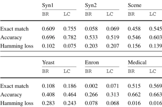
Table 2 displays the performance of the binary relevance BR and label combination LCproblem transformation methods on both synthetic datasets, as well as a selection of real datasets (Scene, Yeast, Enron, and Medical; see e.g. Tsoumakas and Katakis 2007;
Table 2 The performance of the
label-basedBRand example-basedLCproblem transformation methods on the real and synthetic datasets from Table1, under three evaluation measures
Syn1 Syn2 Scene
BR LC BR LC BR LC
Exact match 0.609 0.755 0.058 0.069 0.458 0.545 Accuracy 0.696 0.782 0.533 0.519 0.546 0.603 Hamming loss 0.102 0.075 0.203 0.207 0.156 0.139
Yeast Enron Medical
BR LC BR LC BR LC
Exact match 0.108 0.186 0.002 0.071 0.515 0.569 Accuracy 0.408 0.464 0.266 0.313 0.662 0.663 Hamming loss 0.283 0.243 0.078 0.068 0.016 0.016
Read2010for details), for comparison. These two methods were chosen for their contrast: BR models labels individually and does not explicitly model any dependencies between them, whereasLCmodels labelsets and thus the dependencies between labels. As the base classifier we use Naive Bayes (an incremental classifier). Predictive performance is mea-sured under the evaluation measures described in3.
The variety in the results of Table 2is expected due to the different dimensions and sources of each dataset, but several trends are common throughout: accuracy and exact match is generally higher underLC;BR achieves either higher or comparable Hamming loss toLC; exact match is relatively poorer on data with irregular labelling and a skewed label distribution (Enron, Syn2); and the evaluation statistics all fit within a range—about 0.25 to 0.70 in terms of accuracy. Based on this varied analysis, the synthetic data is indis-tinguishable from the real-world datasets.
It is preferable to use real data whenever it is available, and as interest in mining multi-label data streams continues to rise, more public collections are likely to become available. However, our framework can provide a range of data by using any single-label generation scheme, and analysis indicates that this data is very similar to real-world data and therefore able to serve for general analysis and evaluation of incremental multi-label algorithms. 4.3 Adding concept drift
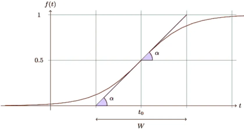
A general framework for modelling concept drift in streaming data was presented in Bifet et al. (2009). This framework uses a sigmoid function (Fig.4) to define the probability that every new instance of a stream belongs to the new concept after the drift. Ifaandbare two data stream concepts, thenc=a⊕W
t0 bis the data stream joining the two streamsaandb,
wheret0is the center of change andW is the number of instances needed to change from one concept to the other.
We can use the same approach in our multi-label stream generator, wherea andbare simply multi-label streams. If these streams are generated with the same random seed and with the same parameters, they will be identical. We add parameterv: the portion of val-ues changed (randomly to different degrees) in the dependency matrixθ after generation. This way we can control subtle changes in label dependencies. For stronger changes in de-pendencies, we can use different random seeds and/or other parameters; both for the label generation, and the underlying single-label generator. This method can be illustrated with a
Fig. 4 A sigmoid functionf (t )=1/(1+e−s(t−t0)), wheres=4 tanα=4/W
simple example; consider streama, of 3 labels, whereπ= [0.2,0.8,0.4], and:
θa= ⎡ ⎣00..20 00..08 00..02 0.0 0.3 0.4 ⎤ ⎦
The multi-label data coming from streamawill have very strong dependencies in the form ofY1being mutually exclusive. Now, let us consider a second streambwhere the concept is changed randomly (this would be parameterv=13on streambi.e. 1/3 of dependencies are changed): θb= ⎡ ⎣00..20 00..08 00..54 1.0 0.3 0.4 ⎤ ⎦
In streamb, the dependencies relating toY3have changed: rather than being mutually exclusive, it now occurs whenever labelY3also occurs. However, the relationships between labelsY1andY2have not changed (this pair is still mutually exclusive). Streamc=a⊕Wt0 b
will represent a shift from conceptato conceptb.
This example is small and rather extreme, but it illustrates how we can make only differ-ent parts of a concept change over time and to a differdiffer-ent degree, if at all. By introducing several changes to the concept (d,e, etc.) we model different changes to different labels at different points in time, and we can specify different types and magnitudes of change; affecting both unconditional and conditional dependencies (the latter naturally involves the attribute space). Because p(y)changes, the mappingζ also changes; thus affecting condi-tional dependencies.
To also change the actual underlying concepts in the data, rather than just the labelling scheme, the parameters of the underlying single-label generator are made different between streams. For example, if we are using the Random Tree Generator (see Sect.7.2), we may change the depth.
In other words, with this generator framework, we have control over the way drift may occur; allowing us to simulate real-world drift in different ways.
5 Dealing with concept drift
Usually the assumption that the data examples are generated from a static distribution does not hold for data streams. Classifiers must therefore adapt to changes in a stream of exam-ples, by incorporating new information and phasing out information when it is no longer relevant. For this, it is important to detect when and where concept drift occurs—and possi-bly also the extent of it, and to do this in real time.
We have already mentioned “batch-incremental” methods, which adapt naturally to con-cept drift by constantly rebuilding classifiers from scratch on new batches of examples (and thus, discarding models built on old potentially-outdated batches). The problem is that, when no drift actually occurs, relevant information is discarded and, with it, possi-ble predictive power. Instance-incremental methods need only to rebuild models when drift occurs—however this makes drift-detection crucial.
Detecting concept drift can, in most cases, be independent of the task of classification. A common strategy is to maintain windows of examples, and to signal a change where two windows differ substantially (for example in terms of error-rate). For multi-label learning, we use the “accuracy” measure which we describe and justify in Sect.3. A modern example of this isADWIN(Bifet and Gavaldà 2007) (ADaptive WINdowing); which maintains an adaptive variably-sized window for detecting concept drift, under the time and memory constraints of the data stream setting. When ADWINdetects change, i.e. a new concept, models built on the previous concept can be discarded.
ADWIN is parameter- and assumption-free in the sense that it automatically detects and adapts to the current rate of change. Its only parameter is a confidence boundδ, indicating how confident we want to be in the algorithm’s output, inherent to all algorithms dealing with random processes.
Also important for our purposes,ADWIN does not maintain the window explicitly, but compresses it using a variant of the exponential histogram technique. This means that it keeps a window of lengthW using onlyO(logW )memory andO(logW )processing time per item.
More precisely, an older fragment of the window is dropped if and only if there is enough evidence that its average value differs from that of the rest of the window. This has two consequences: one, that change is reliably declared whenever the window shrinks; and two, that at any time the average over the existing window can be reliably taken as an estimate of the current average in the stream (barring a very small or very recent change that is still not statistically visible). A formal and quantitative statement of these two points (in the form of a theorem) appears in Bifet and Gavaldà (2007).
6 Multi-label classification methods
In this section, we show how we can use problem transformation methods to build classi-fiers for multi-label data streams, and we present new methods based on using incremental decision tree methods for data streams.
6.1 Using problem transformation methods in data streams
An important advantage of problem transformation is the ability to use any off-the-shelf single-label base classifier to suit requirements. In this section we discuss using incremental base classifiers to meet the requirements of data streams. The methods which we outline
here have been previously discussed and cited in many works, for example, Tsoumakas and Katakis (2007), Read (2010) both give detailed overviews. In this discussion we focus mainly on their possible applications to the data stream context.
6.1.1 Binary relevance (BR)-based methods in data stream settings
Binary Relevance (BR)-based methods are composed of binary classifiers; one for each label. It is straightforward to applyBRto a data stream context by using incremental binary base classifiers.
Some of the advantages ofBRmethods are low time complexity and the ability to run in parallel (in most cases), as well as a resistance to labelset overfitting (since this method learns on a per-label basis). These advantages are also particularly beneficial when learning from data streams.
BRis regarded as achieving poor predictive accuracy, although this can be overcome. For example, in Read et al. (2009) we introduced ensembles ofBR(EBR), and also the concept of classifier-chains (CC), both of which improve considerably overBRin terms of predictive performance.
A problem forBR methods in data streams is that class-label imbalance may become exacerbated by large numbers of training examples. Countermeasures to this are possible, for example by using per-label thresholding methods or classifier weightings as in Ráez et al. (2004).
6.1.2 Label combination (LC)-based methods in data stream settings
The label combination or label power-set method (LC) transforms a multi-label problem into a single-label (multi-class) problem by treating all labelsets (i.e. label combinations) as atomic labels: each unique labelset in the training data is treated as a single label in a single-label multi-class problem.
AlthoughLCis able to model label correlations in the training data and therefore often obtains good predictive performance, its worst-case computational complexity (involving 2Lclasses in the transformed multi-class problem) is a major disadvantage.
A particular challenge forLC-based methods in a data stream context is that the label space expands over timedue to the emergence of new label combinations.
It is possible to adapt probabilistic models to account for the emergence of new labelset combinations over time, however probabilistic models may not necessarily be the best per-forming ones. We instead implement a general ‘buffering’ strategy, where label combina-tions are learned from an initial number of examples and these are considered sufficient to represent the distribution. During the buffering phase, another model can be employed to adhere to the ‘ready to predict at any point’ requirement.
Unfortunately, basicLC must discard any new training examples that have a labelset combination that is not one of the class labels. The pruned sets (PS) method from Read et al. (2008) is anLCmethod much better suited to this incremental learning context: it drastically reduces the number of class-labels in the transformation by pruning all examples with infrequent labelsets (usually a minority). It then additionally subsamples the infrequent labelsets for frequent ones so as to reintroduce examples into the data without reintroducing new labelset combinations.PSthus retains (and often improves upon) the predictive power ofLC, while being up to an order of magnitude faster. Most importantly, its subsampling strategy means that far fewer labelsets are discarded than would be the case underLC. In practice, due to the typical sparsity of labels, hardly any (if any) labelsets are discarded
under PSbecause there almost always exists the possibility to subsample a combination with a single label.
We find that the first 1000 examples are an adequate representation of the labelset dis-tribution of the initial concept.PSstores the first unique labelsets of these 1000 examples with their frequency of occurrence (not necessarily the examples themselves), then builds a PSmodel, and continues to model these labelsets incrementally until the end of the stream or until concept drift is detected (see Sect.5), at which pointPSis reinitialised and buffers again. Values like 500 and 5000 worked similarly as effectively. Higher values letPSlearn a more precise labelset distribution, but leave fewer instances to train on with that distribution, and vice versa for lower values. The range 500–5000 appears to allow a good trade off—we leave more precise analysis for future work. To avoid unusual cases (such as the potential worst case of 21000class labels) we limit the number of unique combinations to the 30 most frequent. On realistic data, we found that this safe-guard parameter has little or no negative effect on predictive performance but can reduce running time significantly. In an ensemble (EPS) any negative effects of buffering are further mitigated by reducing overfitting on the original label space.
We emphasise thatPSin this setup conforms to the requirements of a data stream context. Storing labelset combinations with their frequencies does not entail storing examples, and can be done very efficiently. We use an incremental majority-labelset classifier up until the 1000th example and thus are ready to predict at any point (usingBRduring buffering would be another possibility). Reinitialising a model when concept drift is detected is a standard technique; and is not a limitation ofPS.
6.1.3 Pairwise (PW)-based methods in data stream settings
A binary pairwise classification approach (PW) can also be applied to multi-label classifi-cation as a problem transformation method, where a binary model is trained for each pair of labels, thus modelling a decision boundary between them. AlthoughPWperforms well in several domains and can be adapted naturally to the data stream setting by using incremen-tal base classifiers, as in Fürnkranz et al. (2008), creating decision boundaries between la-bels, instead of modelling their co-occurrence raises doubts and, importantly, faces quadratic complexity in terms of the number of labels and, for this reason, is usually intractable for many data stream problems.
6.2 Multi-label Hoeffding trees (HT)
The Hoeffding tree is the state-of-the-art classifier for single-label data streams, and per-forms prediction by choosing the majority class at each leaf. Predictive accuracy can be increased by adding naive Bayes models at the leaves of the trees. Here, we extend the Hoeffding Tree to deal with multi-label data: a Multi-label Hoeffding Tree.
Hoeffding trees exploit the fact that a small sample can often suffice to choose a splitting attribute. This idea is supported by the Hoeffding bound, which quantifies the number of observations (in our case, examples) needed to estimate some statistics within a prescribed precision (in our case, the goodness of an attribute). More precisely, the Hoeffding bound states that with probability 1−δ, the true mean of a random variable of rangeRwill not differ from the estimated mean afternindependent observations by more than:
= R
2ln(1/δ)
A theoretically appealing feature of Hoeffding trees not shared by other incremental decision tree learners is that it has sound guarantees of performance (Domingos and Hulten2000). Using the Hoeffding bound one can show that its output is asymptotically nearly identical to that of a non-incremental learner using infinitely many examples.
Information gain is a criterion used in leaf nodes to decide if it is worth splitting. In-formation gain for attributeAin a splitting node is the difference between the entropy of the training examplesSat the node and the weighted sum of the entropy of the subsetsSv caused by partitioning on the valuesvof that attributeA.
Info Gain(S, A)=entropy(S)−
v∈A
|Sv|
|S|entropy(Sv)
Hoeffding trees expect that each example belongs to just one class. Entropy is used in C4.5 decision trees and single-label Hoeffding trees for a set of examplesSwithLclasses and probabilityP (c)for each classcas:
entropySL(S)= −
L
i=1
p(ci)log(p(ci))
Clare and King (2001) adapted C4.5 to multi-label data classification by modifying the entropy calculation: entropyML(S)= − L i=1 (p(ci)log(p(ci))+(1−p(ci))log(1−p(ci))) = − L i=1 p(ci)log(p(ci))− L i=1 (1−p(ci))log(1−p(ci)) =entropySL(S)− L i=1 (1−p(ci))log(1−p(ci))
We use their strategy to construct a Hoeffding Tree. A majority-labelset classifier (the multi-label version of majority-class) is used as the default classifier on the leaves of a Multi-label Hoeffding Tree. However, we may use any multi-label classifier at the leaves. Of all the multi-label classifiers that scale well with the size of the data we prefer to use the Pruned Sets method (PS) (Read et al.2008). Reasons for choosing this method over competing ones are presented in the next section.
6.3 Multilabel Hoeffding trees withPSat the leaves (HTP S)
Given the rich availability and strengths of existing methods for multi-label learning which can be applied to data streams (as we have shown in Sect.6), it worth investigating their ef-ficacy ahead of the invention of new incremental algorithms. In this section we detail taking the state of the art in single-label data stream learning (Hoeffding Trees) and combining it with a suitable and effective multi-label method (PS). We demonstrate the suitability of this selection further in Sect.7.
In Sect.6.1.2, we discussed how to useLC-based (e.g.PS) methods in data stream set-tings using a buffering strategy, and thatPSis much more suitable thanLCin this respect. In
the leaves of a Hoeffding Tree, however,PSmay be reset without affecting the core model structure at all, thus creating an even more attractive solution:HTP S.
PSis employed at each leaf of a Hoeffding Tree as we described in Sect.6.1.2. Each new leaf is initialised with a majority labelset classifier. After a number of examples (we allow for 1000) fall into the leaf, aPSclassifier is established to model the combinations observed over these examples, and then proceeds to build this model incrementally with new instances. On smaller datasets, the majority labelset classifier may be in use in many leaves during much of the evaluation. However, we chose 1000 with large data streams in mind.
We emphasise thatHTP S, likeHTandPS(see Sect.6.1.2), meets all the requirements of a data stream learner: it is instance-incremental, does not need to store examples (only a constant number of distinct labelsets are stored at each leaf), and is ready to predict at any point. As described in the following, we wrap it in a bagged ensemble with a change detector to allow adaption to concept drift in an evolving stream.
6.3.1 Ensemble methods
A popular way to achieve superior predictive performance, scalability and parallelization is to use ensemble learning methods, combining several models under a voting scheme to form a final prediction.
When used in an ensemble scheme, any incremental method can adapt to concept drift. We considerADWINBagging (Bifet et al.2009), which is the online bagging method of Oza and Russell (2001) with the addition of theADWIN algorithm as a change detector.
When a change is detected, the worst performing classifier of the ensemble of classifiers is replaced with a new classifier. Algorithm4shows its pseudocode.
Algorithm 4ADWIN Bagging forMmodels
1: Initialize base modelshmfor allm∈ {1,2, . . . , M}
2: for all training examples do
3: form=1,2, . . . , Mdo
4: Setw=Poisson(1)
5: Updatehmwith the current example with weightw
6: ifADWIN detects change in accuracy of one of the classifiers then
7: Replace classifier with lower accuracy with a new one
8: anytime output:
9: return hypothesis:hf in(x)=arg maxy∈Y
T
t=1I (ht(x)=y)
Using this strategy, all the methods we have discussed and presented can adapt to concept drift in evolving data streams, which may include the emergence of new label dependencies.
7 Experimental evaluation
We perform two evaluations: a first comparing several basic problem transformation meth-ods in a data stream environment using Naive Bayes as a base classifier, and a second com-paring newer and more competitive methods with our presented method, using the Hoeffding Tree as a base classifier for problem transformation methods.
The first evaluation shows thatPS is a suitable method to apply on the leaves of the Hoeffding trees, and we use them in the ensemble methods of the second evaluation as our presented method.
7.1 Evaluation measures and methodology
We used evaluation measures and the prequential methodology discussed in Sect.3, using a windoww= N
20 (i.e. the full stream is divided into 20 windows). We display the average of each particular measure across the data windows, and cumulative running time (training plus classification time) in seconds.
The Nemenyi test (Demšar2006) is used for computing significance: it is an appropriate test for comparing multiple algorithms over multiple datasets, being based on the average ranks of the algorithms across all datasets. We use the symbolto indicate statistically significant improvement according to this test. We use ap-value of 0.05. We also supply the algorithms’ per-dataset rankings in parenthesis.
7.2 Datasets
Table 3 provides statistics of our data sources. We chose large multi-label real-world datasets. TMC2007 contains instances of aviation safety reports labelled with problems be-ing described by these reports. We use the version of this dataset specified in Tsoumakas and Vlahavas (2007). IMDB comes from the Internet Movie DataBase; data, where movie plot text summaries are labelled with relevant genres. MediaMill originates from the 2005 NIST TRECVID challenge dataset and contains video data annotated with various concepts. The Ohsumed collection is a subset consisting of peer-reviewed medical articles, labelled with disease categories. Slashdot consists of article blurbs with subject categories, mined from http://slashdot.org. 20NG is the classic 20 newsgroups collection with around 20,000 arti-cles sourced from 20 newsgroups. We also include labelled emails from the Enron dataset; a small collection by data stream standards, but is time-ordered and a superficial analysis shows that it evolves over time. We treat these datasets as a stream by processing them in the order that they were collected. At least in the case of Enron and 20 newsgroups, this represents time order. Read (2010) provides a summary and sources for all these datasets.
For the synthetic data we use two types of generation schemes:
1. The Random Tree Generator (RTG) generator proposed by Domingos and Hulten (2000) produces concepts that in theory should favour decision tree learners. It constructs a decision tree by choosing attributes at random to split, and assigning a random class label to each leaf. Once the tree is built, new examples are generated by assigning uniformly distributed random values to attributes which then determine the class label via the tree. We use a tree depth of 5.
2. The Radial Basis Function (RBF) generator was devised to offer an alternate complex concept type that is not straightforward to approximate with a decision tree model. This generator effectively creates a normally distributed hypersphere of examples surrounding each central point with varying densities. Drift is introduced by moving the centroids with constant speed initialized by a drift parameter. We use two central points for this data. All generation schemes used by our framework are initialised as binary generators. All non-generator specific parameters are inferred from Table3. Three concept drifts of varying type, magnitude, and extent occur in SynT-drift and SynG-drift. For N generated exam-ples, the drifts are centred over examples 1/N, 2/N, and 3/N, extending overN/1000,
Table 3 A sample of seven real
and four synthetic multi-label datasets and their associated statistics
nindicates numeric attributes, andbbinary,φLC(D)is the label cardinality N L A φLC(D) TMC2007 28596 22 500b 2.2 MediaMill 43907 101 120n 4.4 20NG 19300 20 1001b 1.1 IMDB 120919 28 1001b 2.0 Slashdot 3782 22 1079b 1.2 Enron 1702 53 1001b 3.4 Ohsumed 13929 23 1002n 1.7 SynG(g=RBF) 1E5 25 80n 2.8 SynT(g=RTG) 1E6 8 30b 1.6 SynG-drift(g=RBF) 1E5 25 80n 1.5→3.5 SynT-drift(g=RTG) 1E6 8 30b 1.8→3.0
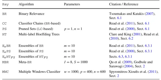
Table 4 Multi-label data stream-capable methods listed with an abbreviation, associated parameters, and
relevant citations and in-paper references
Key Algorithm Parameters Citation / Reference
BR Binary Relevance Tsoumakas and Katakis (2007),
Sect.6.1
CC Classifier Chains (BR-based) Read et al. (2011), Sect.6.1
PS Pruned Sets (LC-based) p=1, n=1 Read et al. (2008), Sect.6.1
HT Multi-label Hoeffding Trees Clare and King (2001), Read et al. (2010), Sect.6.2
EaBR Ensembles ofBR m=10 Read et al. (2011), Sect.6.3.1
EaPS Ensembles ofPS m=10 Read et al. (2008), Sect.6.3.1
EaHTP S Ensembles ofHTP S m=10 Sects.6.3,6.3.1
MBR Meta-BR I=8,S=1000 Qu et al. (2009), Godbole and Sarawagi (2004), Sect.2
MWC Multiple Windows Classifier w=1000, p=400, n=600 Spyromitros-Xioufis et al. (2011), Sect.2
N/100, andN/10 examples, respectively. In the first drift, only 10% of label dependencies change. In the second drift, the underlying concept changes and more labels are associated on average with each example (a higher label cardinality). In the third drift, 20% of label dependencies change. Such types and magnitudes of drift can be found in real world data. Table3provides the basic attributes of the data.
7.3 Methods
Table4lists the methods we use in our experimental evaluation. This table includes the key as used in the results tables, the corresponding algorithm, the parameters used, and relevant citations to the original method as well as references within this paper.
We use the subscriptato denoteADWINmonitoring for concept drift adaption. Therefore BRis an incremental binary classification scheme, andEaBRis an ensemble ofBRwith an ADWINmonitor to detect concept drift. Likewise, EaHTP Sis a baggedADWIN-monitored ensemble of our HTP Smethod (multi-label Hoeffding trees withPSat the leaves).
Table 5 Basic incremental
multi-label methods: accuracy
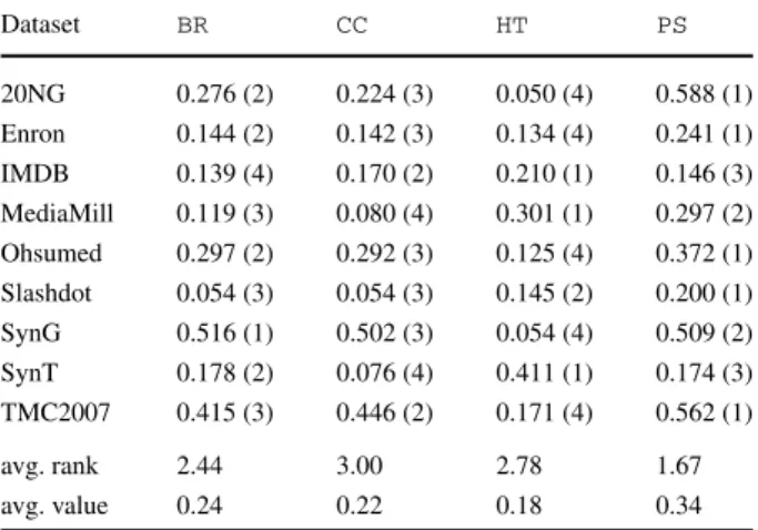
Nemenyi significance:PSCC Dataset BR CC HT PS 20NG 0.276 (2) 0.224 (3) 0.050 (4) 0.588 (1) Enron 0.144 (2) 0.142 (3) 0.134 (4) 0.241 (1) IMDB 0.139 (4) 0.170 (2) 0.210 (1) 0.146 (3) MediaMill 0.119 (3) 0.080 (4) 0.301 (1) 0.297 (2) Ohsumed 0.297 (2) 0.292 (3) 0.125 (4) 0.372 (1) Slashdot 0.054 (3) 0.054 (3) 0.145 (2) 0.200 (1) SynG 0.516 (1) 0.502 (3) 0.054 (4) 0.509 (2) SynT 0.178 (2) 0.076 (4) 0.411 (1) 0.174 (3) TMC2007 0.415 (3) 0.446 (2) 0.171 (4) 0.562 (1) avg. rank 2.44 3.00 2.78 1.67 avg. value 0.24 0.22 0.18 0.34
Note that in Qu et al. (2009) theMBRmethod involved additional strategies to fine tune performance, such as weights to deal with concept drift. This strategy involved nearest-neighbor searching which, as will be shown and explained in the following, would be too costly to add given the already relatively slow performance. The parameters we use for MBRare among those discussed in Qu et al. (2009). We found that other variations (such as
S=500) made negligible difference in relative performance.
ForPS, we use parametersp=1 andn=1; values recommended in Read et al. (2008), and we use the 1000-combination buffering scheme described in Sect.6.1.2. ForMWC’skNN implementation, we setk=11, and used the Jaccard coefficient for distance calculation, as recommended in Spyromitros-Xioufis et al. (2011).
In our experiments, we consider two base classifiers: Naive Bayes for the first set of ex-periments, and Hoeffding trees for the second set. For Hoeffding trees, we use the Hoeffding tree parameters suggested in Domingos and Hulten (2000). ForMBR(in the second set of experiments) we use theWEKA(Hall et al.2009) implementation ofJ482as a suitable base-classifier for comparing decision tree base-classifiers (MBRwas not presented with incremental classifiers).
7.4 Comparing problem transformation methods
In the first of two experimental settings we compared the following methods (all of which were described in Sects.6.1and6.2):BR(the standard baseline), andBR-basedCC,LC -basedPS(similar results toLCbut without the exponential complexity) and multilabelHT. The results, given in Tables5,6,7,8, help support the decision to create a Hoeffding tree classifier withPSat the leaves (introduced in Sect.6.3).
PSperforms best overall. Clearly 1000 examples are sufficient for learning the model in these datasets.
The multi-label Hoeffding trees (HT) generally perform poorly, except on the larger datasets (like IMDB and SynT), where this method suddenly performs very well. An anal-ysis quickly reveals the cause: Hoeffding trees are rather conservative learners and need
Table 6 Basic incremental
multi-label methods: exact match
Nemenyi significance:PSCC Dataset BR CC HT PS 20NG 0.185 (2) 0.040 (4) 0.050 (3) 0.577 (1) Enron 0.006 (4) 0.007 (3) 0.058 (2) 0.086 (1) IMDB 0.031 (2) 0.014 (4) 0.108 (1) 0.027 (3) MediaMill 0.008 (3) 0.000 (4) 0.050 (1) 0.017 (2) Ohsumed 0.115 (2) 0.054 (4) 0.083 (3) 0.212 (1) Slashdot 0.000 (3) 0.000 (3) 0.137 (1) 0.113 (2) TMC2007 0.149 (2) 0.123 (3) 0.087 (4) 0.298 (1) SynG 0.250 (3) 0.271 (2) 0.022 (4) 0.290 (1) SynT 0.039 (4) 0.042 (3) 0.244 (1) 0.099 (2) avg. rank 2.78 3.33 2.22 1.56 avg. value 0.09 0.06 0.09 0.19
Table 7 Basic incremental
multi-label methods: Hamming loss (displayed as 1.0−loss)
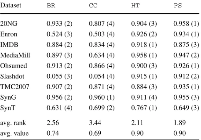
Nemenyi significance:PSCC Dataset BR CC HT PS 20NG 0.933 (2) 0.807 (4) 0.904 (3) 0.958 (1) Enron 0.524 (3) 0.503 (4) 0.926 (2) 0.934 (1) IMDB 0.884 (2) 0.834 (4) 0.918 (1) 0.875 (3) MediaMill 0.897 (3) 0.634 (4) 0.958 (1) 0.947 (2) Ohsumed 0.913 (2) 0.866 (4) 0.900 (3) 0.926 (1) Slashdot 0.055 (3) 0.054 (4) 0.915 (1) 0.912 (2) TMC2007 0.907 (2) 0.871 (4) 0.884 (3) 0.935 (1) SynG 0.956 (2) 0.960 (1) 0.911 (4) 0.955 (3) SynT 0.631 (4) 0.699 (2) 0.767 (1) 0.649 (3) avg. rank 2.56 3.44 2.11 1.89 avg. value 0.74 0.69 0.90 0.90
a considerable number of examples to identify the best split point for a node. As predic-tive performance is averaged over evaluation windows, initial low performance can have an overall negative impact on figures.
As expected, Hoeffding trees excel on SynT which is generated based on tree models. It also performs relatively poorly compared to other methods on SynG which is generated from Gaussian models.
Generally, whenHTcan grow properly, the power of Hoeffding trees can be observed. For any serious application of data streams with a very large number of examples, Hoeffding tree methods are desirable over Naive Bayes, as also discovered by other researchers (e.g. Kirkby2007).
The fact that we expect ever increasing performance from Hoeffding trees with more data does not mean thatPSis unsuitable at the leaves. On the contrary, it tells us that on large datasets (and certain types of data), trees are a better base-classifier option for problem transformation methods. This was part of the reasoning behind our construction of HTP S (Sect.6.3), evaluated in the next section.
Unexpectedly,CCis worse than the baselineBRin several cases. This is almost certainly due to the change in base classifier:CCwas introduced in Read et al. (2011) with Support
Table 8 Basic incremental
multi-label methods: running time (s) Nemenyi significance:HT{BR, CC,PS} Dataset BR CC HT PS 20NG 449 (2) 476 (1) 5 (4) 233 (3) Enron 129 (1) 111 (2) 10 (4) 11 (3) IMDB 5315 (2) 2027 (3) 180 (4) 16243 (1) MediaMill 1069 (1) 861 (2) 71 (4) 361 (3) Ohsumed 438 (2) 457 (1) 15 (4) 409 (3) Slashdot 116 (1) 107 (2) 2 (4) 35 (3) TMC2007 58 (3) 82 (1) 4 (4) 69 (2) SynG 244 (2) 196 (3) 9 (4) 481 (1) SynT 41 (2) 42 (1) 18 (4) 39 (3) avg. rank 1.78 1.78 4.00 2.44 avg. value 873.22 484.33 34.89 1986.78
Vector Machines (SVMs) as a base classifier. Unfortunately SVMs are not a realistic option for instance-incremental learning; and Naive Bayes is clearly a poor choice in terms of predictive performance. Also discussed in Read (2010) is thatCCmay tend to overfit and succumb to class imbalance (along withBR) with large numbers of training instances.
BR-based methods are clearly not suitable for learning from the MediaMill and Slashdot datasets.HTandPSperform much better in these cases.
There is a lot of variation in the results. Methods can differ in performance by 20 percent-age points or more. This would be surprising in a more established area of machine learning, but in the relatively unexplored area of multi-label data streams, there are many unexplored or only partially explored variables, including: the multi-label aspect and the concept-drift detection aspect, thresholding, single-label learner selection, and algorithm parameters. Fur-thermore, on such large datasets, algorithm advantages and disadvantages on different kinds of data become more apparent.
7.5 ComparingEaHTP Sbased methods to state of the art
In this second evaluation we ran experiments comparing our new Hoeffding tree based method (withPSat the leaves:EaHTP S, as introduced in Sect. 6.3) with baseline meth-odsHTaandBRa(‘upgraded’ to use anADWIN monitor for adapting to concept drift), competitive ensemble methods (which we have also adapted to useADWIN) andMBRand MWCfrom the literature. Full results are given in Tables9–13. For measures denoted with↑, lower values are better. Plotting all measures over time for each dataset would be result in too many plots, but we provide Figs.5and6for interests’ sake. Figure7provides details on how often ourADWIN methods detect change for the drifting synthetic datasets.
Our novel method EaHTP S performs overall best under most measures of predictive performance, with the exception of log-loss, and also under exact-match whereHTadoes better. Performance is strongest relative to other methods on the 20NG and OHSU datasets. MBRperforms averagely overall, although does well on the synthetic datasets under ac-curacy, and the smaller real datasets (ENRN, SDOT) under log-loss. It is noteworthy that it does not often improve on the baselineBRaas reported in the paper in which it was intro-duced, which could initially be seen as contradictory—but it is not:BRais usingADWIN to detect change. If there is no change,BRacontinues learning, whereasMBR, as a batch-incremental approach, continuously phases out old information even when it belongs to the current concept. This result is our strongest case for using instance-incremental methods.
Table 9 Adaptive incremental multi-label methods: accuracy
Dataset BRa EaBR EaHTP S EaPS HTa MBR MWC
20NG 0.075 (4) 0.349 (3) 0.542 (1) 0.062 (7) 0.073 (6) 0.075 (5) 0.379 (2) ENRN 0.313 (3) 0.318 (2) 0.157 (4) 0.127 (5) 0.127 (5) 0.109 (7) 0.388 (1) IMDB 0.209 (2) 0.226 (1) 0.134 (6) 0.200 (3) 0.195 (4) 0.160 (5) 0.077 (7) MILL 0.361 (1) 0.361 (2) 0.290 (4) 0.320 (3) 0.265 (5) 0.198 (6) 0.073 (7) OHSU 0.172 (4) 0.293 (2) 0.358 (1) 0.119 (6) 0.119 (6) 0.132 (5) 0.236 (3) SDOT 0.149 (4) 0.176 (3) 0.237 (2) 0.136 (6) 0.137 (5) 0.129 (7) 0.346 (1) SYNG 0.124 (3) 0.418 (2) 0.467 (1) 0.066 (5) 0.051 (6) 0.099 (4) 0.025 (7) SYNG-drift 0.251 (2) 0.272 (1) 0.223 (3) 0.168 (5) 0.178 (4) 0.153 (6) 0.094 (7) SYNT 0.176 (4) 0.178 (3) 0.267 (1) 0.160 (7) 0.160 (6) 0.181 (2) 0.166 (5) SYNT-drift 0.196 (3) 0.195 (4) 0.221 (1) 0.184 (5) 0.164 (6) 0.199 (2) 0.159 (7) TMC7 0.292 (4) 0.419 (2) 0.526 (1) 0.165 (7) 0.170 (6) 0.229 (5) 0.337 (3) avg. rank 3.09 2.27 2.27 5.36 5.36 4.91 4.55 avg. value 0.21 0.29 0.31 0.16 0.15 0.15 0.21
Nemenyi significance:EaBR {EaPS,HTa,MBR};EaHTP S {EaPS,HTa,MBR}
Table 10 Adaptive incremental multi-label methods: exact match
Dataset BRa EaBR EaHTP S EaPS HTa MBR MWC
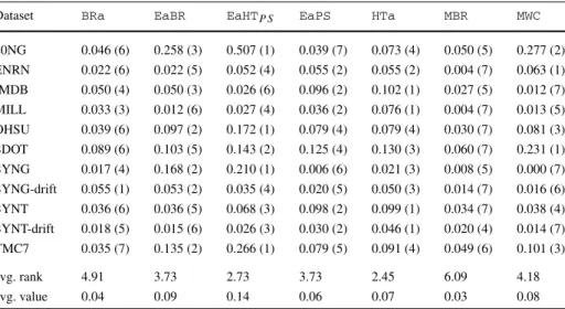
20NG 0.046 (6) 0.258 (3) 0.507 (1) 0.039 (7) 0.073 (4) 0.050 (5) 0.277 (2) ENRN 0.022 (6) 0.022 (5) 0.052 (4) 0.055 (2) 0.055 (2) 0.004 (7) 0.063 (1) IMDB 0.050 (4) 0.050 (3) 0.026 (6) 0.096 (2) 0.102 (1) 0.027 (5) 0.012 (7) MILL 0.033 (3) 0.012 (6) 0.027 (4) 0.036 (2) 0.076 (1) 0.004 (7) 0.013 (5) OHSU 0.039 (6) 0.097 (2) 0.172 (1) 0.079 (4) 0.079 (4) 0.030 (7) 0.081 (3) SDOT 0.089 (6) 0.103 (5) 0.143 (2) 0.125 (4) 0.130 (3) 0.060 (7) 0.231 (1) SYNG 0.017 (4) 0.168 (2) 0.210 (1) 0.006 (6) 0.021 (3) 0.008 (5) 0.000 (7) SYNG-drift 0.055 (1) 0.053 (2) 0.035 (4) 0.020 (5) 0.050 (3) 0.014 (7) 0.016 (6) SYNT 0.036 (6) 0.036 (5) 0.068 (3) 0.098 (2) 0.099 (1) 0.034 (7) 0.038 (4) SYNT-drift 0.018 (5) 0.015 (6) 0.026 (3) 0.030 (2) 0.046 (1) 0.020 (4) 0.014 (7) TMC7 0.035 (7) 0.135 (2) 0.266 (1) 0.079 (5) 0.091 (4) 0.049 (6) 0.101 (3) avg. rank 4.91 3.73 2.73 3.73 2.45 6.09 4.18 avg. value 0.04 0.09 0.14 0.06 0.07 0.03 0.08
Nemenyi significance: {EaHTP S,HTa}MBR
If fully implemented according to Qu et al. (2009) we would expect higher performance fromMBR. However, such an implementation would not be feasible for large data, as we explained in7.3. Already from these results we seeMBRis significantly slower than most other methods.
MWCperforms outstandingly on ENRN and SDOT, often doubling the performance of some of the other methods. This shows the effectiveness of the positive/negative-example balancing method used for theBR-type implementation of this paper. However, on the larger datasets, especially the very large synthetic datasets performance is not as strong (except
![Fig. 2 Combining two binary instances (x +1 and x −1 ) to form a multi-label instance (x ML associated with y = [1, 0, 1, 0, 0]) using mapping ζ](https://thumb-us.123doks.com/thumbv2/123dok_us/778095.2598401/10.659.58.596.75.473/combining-binary-instances-multi-label-instance-associated-mapping.webp)