A Numerical Solution of First order Simultaneous
Fuzzy Differential Equations by Sixth Order
Runge-Kutta Method
P. Rajkumar
1, S. Ruban Raj
21Research Scholar, St. Joseph’s College (Autonomous), Trichy
2Associate Professor (Rtd.), P.G & Research Department of Mathematics, St. Joseph’s College (Autonomous), Trichy, Tamilnadu,
India
Abstract: In this paper we introduce a new technique for getting the approximate solution of “First order Simultaneous Fuzzy differential equation by sixth order Runge-Kutta method” based on Seikkala derivative of fuzzy process [10] in order to increase the order of the accuracy of the solutions. This proposed method is discussed in details followed by a complete error analysis. Keywords: Cauchy Problem - Runge-Kutta sixth order Method – First order simultaneous fuzzy differential equation – Error Analysis
I. INTRODUCTION
The concept of fuzzy derivatives was first introduced by S.L. Chang and L.A. Zadeh [6], it was followed up by D. Dubois and Prade [7] who used the extension principle in their approach. Puri and D.A. Ralesec [15] and R. Goetschel and W. Voxman [9] contributed towards the differential of fuzzy functions.
The fuzzy differential equation and initial value problems were extensively studied by O. Kaleva [10, 11] and by S. Seikkala [16]. Numerical solution of fuzzy differential equations has been introduced by M. Ma, M. Friedman, A. Kandel [13] through Euler method and by S. Abbasbandy and T. Allahviranloo [1] by Taylor method. Runge-Kutta methods have also been studied by authors [2, 14].
In this paper organized as follows: In Section 2, some basic definitions and results on fuzzy numbers and fuzzy derivatives. Section 3 contains the definition of fuzzy Cauchy problem with initial conditions. Section 4, discussed about sixth order Runge-Kutta method and defined to solve the first order simultaneous fuzzy differential equation with initial value problem. The proposed method is illustrated and solved the numerical example in section 5, also the result is compared with Euler’s method and Runge-Kutta fourth order method with the approximation solution by Runge-Runge-Kutta sixth order method.
II. PRELIMINARIES
Consider the first order simultaneous differential equation
)
,
,
(
d
z
y
t
f
dt
y
&
dz
g
(
t
,
y
,
z
)
dt
, t0 t b, initial conditions y(t0) = y0, z(t0) = z0. . . (2.1) The basis of all Runge-Kutta methods is to express the difference between the value of y at tn+1 and tn as
m
i i i n
n
y
w
k
y
0
1 ; where wi are constant i and
ki = hf(tn+aih, yn +
1
1
i
j j ij
k
c
)Consider
y(tn+1) = y(tn) + w1k1 + w2k2 + w3k3 + w4k4 + w5k5 + w6k6 + w7k7 where
k1 = h f(tn, y(tn))
k2 = h f(tn+c2h, y(tn)+a21k1) k3 = h f(tn+c3h, y(tn)+a31k1+a32k2) k4 = h f(tn+c4h, y(tn)+a41k1+a42k2+a43k3) k5 = h f(tn+c5h, y(tn)+a51k1+a52k2+a53k3+a54k4)
k6 = h f(tn+c6h, y(tn)+a61k1+a62k2+a63k3+a64k4+a65k5+a66k6)
k7 = h f(tn+c7h, y(tn)+a71k1+a72k2+a73k3+a74k4 + a75k5+a76k6 + a77k7) . . . (2.2) Utilizing the Taylor’s series expansion techniques, Runge-Kutta method of order sixth is given by,
yn+1 = yn +
180
9
49
49
64
9
k
1
k
3
k
5
k
6
k
7where
k1 = h f(tn, y(tn))
k2 = h f(tn+ vh, y(tn)+ vk1)
k3 = h f(tn+
2
h
, y(tn)+ ((4v – 1)k1 + k2)/(8v))
k4 = h f(tn+
3
2
h
, y(tn)+((10v – 2)k1 + 2k2 + 8vk3)/(27v))
k5 = h f(tn+(7+4.582576)
14
h
, y(tn)+(-((77v–56)+(17v–8)4.582576)k1–8(7+4.582576)k2
+ 48(7+4.582576)vk3 – 3(21+4.582576)vk4)/(392v)
k6 = h f(tn+(7 - 4.582576)
14
h
, y(tn)+(-5((287v–56) - (59v–8)4.582576)k1–40(7-4.582576)k2
+ 320(4.582576)vk3 + 3(21-121(4.582576))vk4 + 392(6-4.582576)vk5) /(1960v)
k7 = h f(tn + h, y(tn) + (15((30v – 8) - 7v(4.582576))k1+120k2 – 40(5 + 7(4.582576))vk3 + 63(2 + 3(4.582576))vk4 – 14(49 - 9(4.582576))vk5 + 70(7 + 4.582576)vk6)/(180v)
. . . (2.3) and
zn+1 = zn +
180
9
49
49
64
9
l
1
l
3
l
5
l
6
l
7where
l1 = h g(tn, z(tn))
l2 = h g(tn+ vh, z(tn)+ vl1)
l3 = h g(tn+
2
h
, z(tn)+ ((4v – 1)l1 + l2)/(8v))
l4 = h g(tn+
3
2
h
, z(tn)+((10v – 2)l1 + 2l2 + 8vl3)/(27v))
l5 = h g(tn+(7+4.582576)
14
h
, z(tn)+(-((77v–56)+(17v–8)4.582576)l1–8(7+4.582576)l2
+ 48(7+4.582576)vl3 – 3(21+4.582576)vl4)/(392v)
l6 = h g(tn+(7 - 4.582576)
14
h
+ 320(4.582576)vl3 + 3(21-121(4.582576))vl4 + 392(6-4.582576)vl5) /(1960v)
l7 = h g(tn + h, z(tn) + (15((30v – 8) - 7v(4.582576))l1+120l2 – 40(5 + 7(4.582576))vl3 + 63(2 + 3(4.582576))vl4 – 14(49 - 9(4.582576))vl5 + 70(7 + 4.582576)vl6)/(180v)
. . . (2.4)
A. Definition – 2.1
A fuzzy number u as a fuzzy subset of R ie) u : R [0, 1] satisfying the following conditions.
1) u is normal, ie x0R u(x0) = 1
2) u is a convex fuzzy set
ie) u(tx + (1-t)y) min{u(x), u(y)}, t [0, 1] and x, y R
3) u is upper semi continuous on R
4)
x
R
,
u
x
0
is compactThe set E is the family of fuzzy numbers and arbitrary fuzzy number is represented by an ordered pair of functions
u
r
,
u
r
, 0 r 1 has satisfies the following requirements
a)
u
r
is a bounded left continuous non-decreasing function over [0, 1] with respect to any ‘r’.b)
u
r
is a bounded right continuous non-increasing function over [0, 1] with respect to any ‘r’.c)
u
r
u
r
, 0 r 1, r-level cut is [u]r = {x/u(x) r}, 0 r 1 as a closed & bounded interval denoted by [u]r =
u
r
,
u
r
and clearly [u]0 = {x/u(x) > 0} is compact.B. Definition – 2.2
A triangular fuzzy number u is a fuzzy set in E that is characterised by an ordered triple (ul, uc, ur)R3 with ul <uc <ur such that [u]0 = [ul : ur] and [u]1 = [uc]. The membership function of the triangular fuzzy number u is given by
r c
c r
r
c c l
l c
l
u
x
u
u
u
x
u
u
x
u
x
u
u
u
u
x
x
u
,
1
,
and we will have . . . (2.4)
i). u > 0 if ul> 0 ii). u 0 if ul 0 iii). u < 0 if uc < 0 iv). u 0 if uc 0
Let I be a real interval. A mapping y : I E as called a fuzzy process and its - level set is denoted by
y
t
y
t
,
y
,
y
t
,
y
, t I, 0 < I,
z
t
z
t
,
z
,
z
t
,
z
, t I, 0 < I.The Seikkala derivative y(t) of a fuzzy process is defined by
y
t
y
t
,
y
,
y
t
,
y
1 1
1
, t I, 0 < I provided the equation
defines fuzzy number as in [11]. Similarly, let I be a real interval. A mapping z: IE is called a fuzzy process and its - level set
is denoted by
z
t
z
t
,
y
,
z
,
z
t
,
y
,
z
, t I, 0 < I. For u, v E and , the u + v and the product u can be defined by [u + v] = [u] + [v] and [u] = [u], where [0, 1] and [u] + [v] means the addition of two intervals of and[u] means the product between a scalar and a subset of .
i). u = v if
u
r
v
r
andu
r
v
r
ii). u + v =
u
r
v
r
,
u
r
v
r
iii). u - v =
u
r
v
r
,
u
r
v
r
iv). u =
u
r
,
u
r
if 0 =
u
r
,
u
r
if < 0III. A FUZZY CAUCHY PROBLEM
Consider the first order simultaneous differential equation
)
,
,
(
d
z
y
t
f
dt
y
&
dz
g
(
t
,
y
,
z
)
dt
, t0 t b, initial conditions y(t0) = y0, z(t0) = z0Let the function f be a continuous mapping from R x R R and y0 E with r-level sets [y0]r =
y
0
:
r
,
y
0
:
r
, r [0, 1] andthe function g be a continuous mapping from R x R R and z0 E with r-level sets [z0]r =
z
0
:
r
,
z
0
:
r
, r [0, 1]. The extension principle of Zadeh [4] leads to the definition of f(t, y, z) and g(t, y, z), y = y(t), z = z(t) are the fuzzy numbers.
f
t
,
y
,
z
r
f
t
,
y
,
z
:
r
,
f
t
,
y
,
z
:
r
, r[0, 1], It follows that
t
y
z
r
f
t
u
v
u
y
r
y
r
v
z
r
z
r
f
,
,
:
min
,
,
,
,
,
t
y
z
r
f
t
u
v
u
y
r
y
r
v
z
r
z
r
f
,
,
:
max
,
,
,
,
,
. . . (3.1) and
t
y
z
r
g
t
u
v
u
y
r
y
r
v
z
r
z
r
g
,
,
:
min
,
,
,
,
,
t
y
z
r
g
t
u
v
u
y
r
y
r
v
z
r
z
r
g
,
,
:
max
,
,
,
,
,
. . . (3.2)
A. Theorem
Let f satisfy
f
t
,
v
f
t
,
v
g
t
,
v
v
, t 0 and v,v R, . . . (3.3)where g : R+ x R+ R+ is a continuous mapping such that r g(t, r) is non-decreasing an initial value problem u1(t) = g(t, u(t)), u(0) = u0 ... (3.3) has a solution on R+ or u0 > 0 and that u(t) 0 is the only solution of (3.3) for u0 = 0 then the fuzzy initial value problem has a unique fuzzy solution.
Proof : See [16].
IV. FUZZY SIXTH ORDER RUNGE–KUTTA METHOD
Let the exact solution of the given equation [Y(t)]r =
Y
t
:
r
,
Y
t
:
r
is approximated by some solution [y(t)]r =
y
t
:
r
,
y
t
:
r
and the exact solution of the given equation [Z(t)]r =
Z
t
:
r
,
Z
t
:
r
is approximated by some solution[z(t)]r =
z
t
:
r
,
z
t
:
r
also we define
7
1
1
:
:
i i i n
n
r
y
t
r
w
k
t
y
7
1
1
:
:
i i i n
n
r
y
t
r
w
k
t
y
where wi’s are constant
t
y
t
r
hf
t
y
t
r
k
1,
:
n,
n:
k
1
t
,
y
t
:
r
hf
t
n,
y
t
n:
r
12
,
:
2
:
,
y
t
r
hf
t
h
y
t
r
v
k
t
k
n n
12
,
:
2
:
,
y
t
r
hf
t
h
y
t
r
v
k
t
k
n n
hf
t
h
y
t
r
v
k
k
v
r
t
y
t
k
n,
n:
4
1
/
8
2
:
,
1 23
hf
t
h
y
t
r
v
k
k
v
r
t
y
t
k
n,
n:
4
1
/
8
2
:
,
1 23
hf
t
h
y
t
r
v
k
k
v
k
v
r
t
y
t
k
n,
n:
10
2
2
8
/
27
3
2
:
,
1 2 34
hf
t
h
y
t
r
v
k
k
v
k
v
r
t
y
t
k
n,
n:
10
2
2
8
/
27
3
2
:
,
1 2 34
v k v k v k k v v r t y h t hf r t y tk n n /392
582576 . 4 21 3 582576 . 4 7 48 582576 . 4 7 8 582576 . 4 8 17 56 77 : , 14 582576 . 4 7 : , 4 3 2 1 5
v k v k v k k v v r t y h t hf r t y tk n n /392
582576 . 4 21 3 582576 . 4 7 48 582576 . 4 7 8 582576 . 4 8 17 56 77 : , 14 582576 . 4 7 : , 4 3 2 1 5
v
k
v
k
v
k
v
k
k
v
v
r
t
y
h
t
hf
r
t
y
t
k
n n/
1960
582576
.
4
6
392
582576
.
4
121
21
3
582576
.
4
320
582576
.
4
7
40
582576
.
4
8
59
56
287
5
:
,
14
582576
.
4
7
:
,
5 4 3 2 1 6
v
k
v
k
v
k
v
k
k
v
v
r
t
y
h
t
hf
r
t
y
t
k
n n/
1960
582576
.
4
6
392
582576
.
4
121
21
3
582576
.
4
320
582576
.
4
7
40
582576
.
4
8
59
56
287
5
:
,
14
582576
.
4
7
:
,
5 4 3 2 1 6
v k v k v k v k v k k v v r t y h t hf r t y tk n n /180
582576 . 4 7 70 582576 . 4 9 49 14 582576 . 4 3 2 63 582576 . 4 7 5 40 120 582576 . 4 7 8 30 15 : , : , 6 5 4 3 2 1 7
v k v k v k v k v k k v v r t y h t hf r t y tk n n /180
582576 . 4 7 70 582576 . 4 9 49 14 582576 . 4 3 2 63 582576 . 4 7 5 40 120 582576 . 4 7 8 30 15 : , : , 6 5 4 3 2 1 7
. . . (4.1) also define
7 11
:
:
i i i n
n
r
z
t
r
w
l
t
z
7 1
1
:
:
i i i n
n
r
z
t
r
w
l
t
z
where li’s are constant
where
t
z
t
r
hg
t
z
t
r
l
1,
:
n,
n:
l
1
t
,
z
t
:
r
hg
t
n,
z
t
n:
r
12
,
:
2
:
,
z
t
r
hg
t
h
z
t
r
v
l
t
l
n n
12
,
:
2
:
,
z
t
r
hg
t
h
z
t
r
v
l
t
l
n n
hg
t
h
z
t
r
v
l
l
v
r
t
z
t
l
n,
n:
4
1
/
8
2
:
,
1 23
hg
t
h
z
t
r
v
l
l
v
r
t
z
t
l
n,
n:
4
1
/
8
2
:
,
1 23
hg
t
h
z
t
r
v
l
l
v
l
v
r
t
z
t
l
n,
n:
10
2
2
8
/
27
3
2
:
,
1 2 34
h
t
h
z
t
r
v
l
l
v
l
v
r
t
z
t
l
n,
n:
10
2
2
8
/
27
3
2
:
,
1 2 34
v l v l v l l v v r t z h t hg r t z tl n n /392
582576 . 4 21 3 582576 . 4 7 48 582576 . 4 7 8 582576 . 4 8 17 56 77 : , 14 582576 . 4 7 : , 4 3 2 1 5
v l v l v l l v v r t z h t hg r t z tl n n /392
582576 . 4 21 3 582576 . 4 7 48 582576 . 4 7 8 582576 . 4 8 17 56 77 : , 14 582576 . 4 7 : , 4 3 2 1 5
v
l
v
l
v
l
v
l
l
v
v
r
t
z
h
t
hg
r
t
z
t
l
n n/
1960
582576
.
4
6
392
582576
.
4
121
21
3
582576
.
4
320
582576
.
4
7
40
582576
.
4
8
59
56
287
5
:
,
14
582576
.
4
7
:
,
5 4 3 2 1 6
v
l
v
l
v
l
v
l
l
v
v
r
t
z
h
t
hg
r
t
z
t
l
n n/
1960
582576
.
4
6
392
582576
.
4
121
21
3
582576
.
4
320
582576
.
4
7
40
582576
.
4
8
59
56
287
5
:
,
14
582576
.
4
7
:
,
5 4 3 2 1 6
v l v l v l v l v l l v v r t z h t hg r t z tl n n /180
582576 . 4 7 70 582576 . 4 9 49 14 582576 . 4 3 2 63 582576 . 4 7 5 40 120 582576 . 4 7 8 30 15 : , : , 6 5 4 3 2 1 7
v l v l v l v l v l l v v r t z h t hg r t z tl n n /180
582576 . 4 7 70 582576 . 4 9 49 14 582576 . 4 3 2 63 582576 . 4 7 5 40 120 582576 . 4 7 8 30 15 : , : , 6 5 4 3 2 1 7
. . . (4.2)
180
:
,
7
9
:
,
6
49
:
,
5
49
:
,
3
64
:
,
1
9
:
,
r
t
y
t
k
r
t
y
t
k
r
t
y
t
k
r
t
y
t
k
r
t
y
t
k
r
t
y
t
G
and
180
:
,
7
9
:
,
6
49
:
,
5
49
:
,
3
64
:
,
1
9
:
,
r
t
z
t
l
r
t
z
t
l
r
t
z
t
l
r
t
z
t
l
r
t
z
t
l
r
t
z
t
P
180
:
,
7
9
:
,
6
49
:
,
5
49
:
,
3
64
:
,
1
9
:
,
r
t
z
t
l
r
t
z
t
l
r
t
z
t
l
r
t
z
t
l
r
t
z
t
l
r
t
z
t
Q
The exact and the approximate solution of the differential equation at tn, 0 n N are denoted by [Y(tn)]r =
Y
t
n:
r
,
Y
t
n:
r
, [y(tn)]r =
y
t
n:
r
,
y
t
n:
r
and [Z(tn)]r =
Z
t
n:
r
,
Z
t
n:
r
, [z(tn)]r =
z
t
n:
r
,
z
t
n:
r
respectively. Therefore we have
t
r
Y
t
r
F
t
Y
t
r
Y
n1:
n:
n,
n:
Y
t
n1:
r
Y
t
n:
r
G
t
n,
Y
t
n:
r
t
r
Z
t
r
P
t
Z
t
r
Z
n1:
n:
n,
n:
Z
t
n1:
r
Z
t
n:
r
Q
t
n,
Z
t
n:
r
t
r
y
t
r
F
t
y
t
r
y
n1:
n:
n,
n:
y
t
n1:
r
y
t
n:
r
G
t
n,
y
t
n:
r
t
r
z
t
r
P
t
z
t
r
z
n1:
n:
n,
n:
z
t
n1:
r
z
t
n:
r
Q
t
n,
z
t
n:
r
. . (4.3) To show the convergence of these approximation of y is
ie)
y
t
r
Y
t
r
h
:
:
lim
0
and
t
r
Y
t
r
y
h
:
:
lim
0
Similarly, To show the convergence of these approximation of y is ie)
z
t
r
Z
t
r
h
:
:
lim
0
and
t
r
Z
t
r
z
h
:
:
lim
0
A. Lemma
Let a sequence of numbers
W
Nn0 satisfy1
n
W
AW
n + B, 0 n N – 1 or some given positive constants A and B thenn
W
An0
W
+B1
1
A
A
n, 0 n N–1
Proof : See [13]
B. Lemma
Let a sequence of numbers
W
Nn0 and
V
nN0 satisfy the condition1
n
W
W
n + A max
W
n,
V
n
B
and1
n
Proof : See [13]
C. Theorem
Let F(t, u, v) and G(t, u, v) belongs to C4(K) and let the partial derivatives of F and G be bounded over K, then for arbitrary fixed value r, 0 r 1 are approximate solutions converge to the exact solutions of
Y
t
n:
r
andY
t
n:
r
uniformly in t.Proof : See [13]
V. NUMERICAL EXAMPLE
Consider the first order simultaneous differential equation
z
y
dt
y
4
3
d
andz
y
dt
2
3
dz
Fuzzy initial conditions arey(0) = (3.8 + 0.2r, 4.25-0.25r) and z(0) = (2.75 + 0.25r, 3.2-0.2r); 0 ≤ r ≤ 1.
Solution:
The exact solution of y is
Y
(
t
:
r
)
2
y
1
t
:
r
e
t
y
2
t
:
r
e
tand the exact solution of z is
t
te
r
t
z
e
r
t
z
r
t
Z
(
:
)
1:
2:
when t = 1 then the exact solution is given by,0.2r)e
+
(1.8
0.15r)e
+
2(0.85
)
:
1
(
r
-1
Y
Y
(
1
:
r
)
2(1.2
-
0.2r)e
-1
(2.25
-
0.25r)e
ande
e
r
Z
(
1
:
)
(0.75
+
0.25r)
1
(1.85
+
0.15r)
Z
(
1
:
r
)
(1.25
-
0.25r)e
-1
(2.3
-
0.3r)e
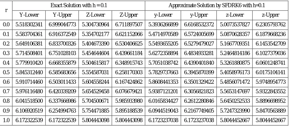
[image:8.595.39.534.469.685.2]The exact and approximate solutions for the first order simultaneous fuzzy differential equation obtained by the Runge-Kutta sixth order method for taking h = 0.1
Table – 5.1 Comparison between Exact and SFDRK6 Solution
r Exact Solution with h = 0.1 Approximate Solution by SFDRK6 with h=0.1
Y-Lower Y-Upper Z-Lower Z-Upper y-Lower y-Upper z-Lower z-Upper
0.0 5.518302341 6.999044773 5.304730964 6.711897507 5.3936266899 6.6168532372 5.0073537827 6.2305793762
0.1 5.583704361 6.916372549 5.354702177 6.621152066 5.4714970589 6.5724005699 5.0870628357 6.1879668236
0.2 5.649106381 6.833700326 5.404673390 6.530406625 5.5493655205 6.5279479027 5.1667709351 6.1453542709
0.3 5.714508401 6.751028103 5.454644604 6.439661184 5.6272358894 6.4834933281 5.2464814186 6.1027379036
0.4 5.779910420 6.668355879 5.504615817 6.348915743 5.7051038742 6.4390401840 5.3261880875 6.0601248741
0.5 5.845312440 6.585683656 5.554587031 6.258170303 5.7829737663 6.3945870399 5.4058976173 6.0175104141
0.6 5.910714460 6.503011433 5.604558244 6.167424862 5.8608441353 6.3501329422 5.4856071472 5.9748954773
0.7 5.976116480 6.420339209 5.654529458 6.076679421 5.9387121201 6.3056821823 5.5653147697 5.9322843552
0.8 6.041518500 6.337666986 5.704500671 5.985933980 6.0165834427 6.2612280846 5.6450252533 5.8896698952
0.9 6.106920519 6.254994763 5.754471885 5.895188539 6.0944519043 6.2167749405 5.7247323990 5.8470563889
1.0 6.172322539 6.172322539 5.804443098 5.804443098 6.1723237038 6.1723237038 5.8044452667 5.8044452667
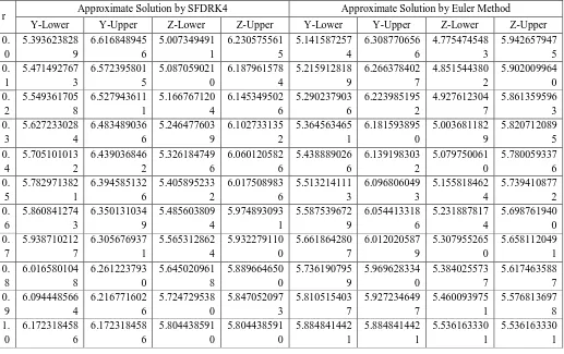
Table – 5.2 Solution of SFDE by SFDRK4 and Euler’s Method
r Approximate Solution by SFDRK4 Approximate Solution by Euler Method Y-Lower Y-Upper Z-Lower Z-Upper Y-Lower Y-Upper Z-Lower Z-Upper 0.
0
5.393623828 9
6.616848945 6
5.007349491 1
6.230575561 5
5.141587257 4
6.308770656 6
4.775474548 3
5.942657947 5 0.
1
5.471492767 3
6.572395801 5
5.087059021 0
6.187961578 4
5.215912818 9
6.266378402 7
4.851544380 2
5.902009964 0 0.
2
5.549361705 8
6.527943611 1
5.166767120 4
6.145349502 6
5.290237903 6
6.223985195 2
4.927612304 7
5.861359596 3 0.
3
5.627233028 4
6.483489036 6
5.246477603 9
6.102733135 2
5.364563465 1
6.181593895 0
5.003681182 9
5.820712089 5 0.
4
5.705101013 2
6.439036846 2
5.326184749 6
6.060120582 6
5.438889026 6
6.139198303 2
5.079750061 0
5.780059337 6 0.
5
5.782971382 1
6.394585132 6
5.405895233 2
6.017508983 6
5.513214111 3
6.096806049 3
5.155818462 4
5.739410877 2 0.
6
5.860841274 3
6.350131034 9
5.485603809 4
5.974893093 1
5.587539672 9
6.054413318 6
5.231887817 4
5.698761940 0 0.
7
5.938710212 7
6.305676937 1
5.565312862 4
5.932279110 0
5.661864280 7
6.012020587 9
5.307955265 0
5.658112049 1 0.
8
6.016580104 8
6.261223793 0
5.645020961 8
5.889664650 0
5.736190795 9
5.969628334 0
5.384025573 7
5.617463588 7 0.
9
6.094448566 4
6.216771602 6
5.724729538 0
5.847052097 3
5.810515403 7
5.927234649 7
5.460093975 1
5.576813697 8 1.
0
6.172318458 6
6.172318458 6
5.804438591 0
5.804438591 0
5.884841442 1
5.884841442 1
5.536163330 1
5.536163330 1
Table – 5.3 Complete Error Analysis
5 5.2 5.4 5.6 5.8 6 6.2 6.4 6.6 6.8 7
[image:9.595.46.563.396.721.2]r
Error in SFDRK6 Method Error in Euler Method Error in SFDRK4 Method
Y-Lower Y-Upper
y-Lower
Z-Upper
y-Lower
y-Upper
z-Lower
z-Upper
y-Lower
y-Upper
z-Lower
z-Upper 0.
0
0.1246 76
0.3821 92
0.2973 77
0.4813 18
0.3767 15
0.6902 74
0.5292 56
0.7692 40
0.1246 79
0.3821 96
0.2973 81
0.4813 22 0.
1
0.1122 07
0.3439 72
0.2676 39
0.4331 85
0.3677 92
0.6499 94
0.5031 58
0.7191 42
0.1122 12
0.3439 77
0.2676 43
0.4331 90 0.
2
0.0997 41
0.3057 52
0.2379 02
0.3850 52
0.3588 68
0.6097 15
0.4770 61
0.6690 47
0.0997 45
0.3057 57
0.2379 06
0.3850 57 0.
3
0.0872 73
0.2675 35
0.2081 63
0.3369 23
0.3499 45
0.5694 34
0.4509 63
0.6189 49
0.0872 75
0.2675 39
0.2081 67
0.3369 28 0.
4
0.0748 07
0.2293 16
0.1784 28
0.2887 91
0.3410 21
0.5291 58
0.4248 66
0.5688 56
0.0748 09
0.2293 19
0.1784 31
0.2887 95 0.
5
0.0623 39
0.1910 97
0.1486 89
0.2406 60
0.3320 98
0.4888 78
0.3987 69
0.5187 59
0.0623 41
0.1910 99
0.1486 92
0.2406 61 0.
6
0.0498 70
0.1528 78
0.1189 51
0.1925 29
0.3231 75
0.4485 98
0.3726 70
0.4686 63
0.0498 73
0.1528 80
0.1189 54
0.1925 32 0.
7
0.0374 04
0.1146 57
0.0892 15
0.1443 95
0.3142 52
0.4083 19
0.3465 74
0.4185 67
0.0374 06
0.1146 62
0.0892 17
0.1444 00 0.
8
0.0249 35
0.0764 39
0.0594 75
0.0962 64
0.3053 28
0.3680 39
0.3204 75
0.3684 70
0.0249 38
0.0764 43
0.0594 80
0.0962 69 0.
9
0.0124 69
0.0382 20
0.0297 39
0.0481 32
0.2964 05
0.3277 60
0.2943 78
0.3183 75
0.0124 72
0.0382 23
0.0297 42
0.0481 36 1.
0
0.0000 01
0.0000 01
0.0000 02
0.0000 02
0.2874 81
0.2874 81
0.2682 80
0.2682 80
0.0000 04
0.0000 04
0.0000 05
0.0000 05
VI. CONCLUSION
In this work, we have used the proposed fuzzy sixth order Runge-Kutta method to find the numerical solution of simultaneous fuzzy differential equations. Taking into account the convergence order of the Euler method is O(h), a higher order of convergence O(h3) is obtained by the proposed method and by the method proposed in [14]. Comparison of the solutions of example 5 shows that the proposed method gives a better solution than the Euler method and by the Runge-Kutta fourth order method.
REFERENCES
[1] Abbasbandy.S, Allah Viranloo.T (2002), “Numerical Solution of fuzzy differential equations by Taylor’s method”, Journal of Computational Methods in Applied Mathematics 2(2), pp 113-124
[2] Abbasbandy.S, Allah Viranloo.T (2004), “Numerical Solution of fuzzy differential equations by Runge-Kutta method”, Nonlinear Studies 11(1), pp 117-129 [3] Buckley.J.J, Eslami.E, and Feuring.T (2002), “Fuzzy Mathematics in Economics and Engineering”, Heidelberg, Germany, Physics-Verla
[4] Buckley.J.J, Feuring.T (2000), “Fuzzy Differential Equations”, Fuzzy Sets and Systems 110, pp 43-54
[5] Butcher.J.C (1987), “The Numerical Analysis of Ordinary Differential Equations by Runge-Kutta and General Linear Methods”, New York, Wiley [6] Chang.S.L, Zadeh.L.A (1972), “On fuzzy mapping and Control”, IEEE Transactions on System Man Cybernetics 2(1), pp 30-34
[7] Dubois.D, Prade.H (1982), “Towards Fuzzy Differential Calculus : Part 3, Differentiation”, Fuzzy Sets and System 8, pp 225-233 [8] Goeken.D, Johnson (2000), “Runge-Kutta with higher order derivative Approximations”, Applied Numerical Mathematics 34, pp 207-218 [9] Goetschel.R, Voxman.W (1986), “Elementary Fuzzy Calculus”, Fuzzy Sets and Systems 18, pp 31-43
[10] Kaleva.O(1987),“Fuzzy Differential Equations”,Fuzzy Sets & Systems 24, pp 301-317
[11] Kaleva.O (1990), “The Cauchy’s problem for Ordinary differential equations”, Fuzzy Sets and Systems 35, pp 389-396 [12] Lambert.J.D (1990), “Numerical methods for Ordinary differential systems’, New York, Wiley
[13] Ma.M, Friedman.M, Kandel.A (1999), “Numerical solution of Fuzzy differential Equations”, Fuzzy Sets and System 105, pp 133-138
[14] Palligkinis.S,Ch., Papageorgiou.G, Famelis.I.TH (2009), “Runge-Kutta methods for fuzzy differential equations”, Applied Mathematics Computation 209, pp 97-105