RIT Scholar Works
RIT Scholar Works
Theses11-2019
Computational Methods for Segmentation of Modal
Computational Methods for Segmentation of Modal
Multi-Dimensional Cardiac Images
Dimensional Cardiac Images
Shusil Dangi
Follow this and additional works at: https://scholarworks.rit.edu/theses
Recommended Citation Recommended Citation
Dangi, Shusil, "Computational Methods for Segmentation of Multi-Modal Multi-Dimensional Cardiac Images" (2019). Thesis. Rochester Institute of Technology. Accessed from
This Dissertation is brought to you for free and open access by RIT Scholar Works. It has been accepted for inclusion in Theses by an authorized administrator of RIT Scholar Works. For more information, please contact
by
Shusil Dangi
A dissertation submitted in partial fulfillment of the requirements for the degree of Doctor of Philosophy in the Chester F. Carlson Center for Imaging Science
College of Science
Rochester Institute of Technology
November 2019
c
by
Shusil Dangi
B.E. Pulchowk Campus, Institute of Engineering, Tribhuvan University, 2011
A dissertation submitted in partial fulfillment of the requirements for the degree of Doctor of Philosophy in the Chester F. Carlson Center for Imaging Science
College of Science
Rochester Institute of Technology 2019
Signature of the Author
Accepted by
CERTIFICATE OF EXAMINATION
Advisor Committee
Dr. Cristian A. Linte Dr. Nathan D. Cahill
Dr. Christopher Kanan
Dr. Ziv Yaniv
The dissertation by Shusil Dangi
entitled
Computational Methods for Segmentation of Multi-Modal Multi-Dimensional Cardiac Images
is accepted in partial fulfillment of the requirements for the degree of
Doctor of Philosophy in Imaging Science
Date
Segmentation of the heart structures helps compute the cardiac contractile func-tion quantified via the systolic and diastolic volumes, ejecfunc-tion fracfunc-tion, and myocardial mass, representing a reliable diagnostic value. Similarly, quantification of the my-ocardial mechanics throughout the cardiac cycle, analysis of the activation patterns in the heart via electrocardiography (ECG) signals, serve as good cardiac diagnosis indicators. Furthermore, high quality anatomical models of the heart can be used in planning and guidance of minimally invasive interventions under the assistance of image guidance.
The most crucial step for the above mentioned applications is to segment the ven-tricles and myocardium from the acquired cardiac image data. Although the manual delineation of the heart structures is deemed as the gold-standard approach, it re-quires significant time and effort, and is highly susceptible to inter- and intra-observer variability. These limitations suggest a need for fast, robust, and accurate semi- or fully-automatic segmentation algorithms. However, the complex motion and anatomy of the heart, indistinct borders due to blood flow, the presence of trabeculations, in-tensity inhomogeneity, and various other imaging artifacts, makes the segmentation task challenging.
In this work, we present and evaluate segmentation algorithms for multi-modal, multi-dimensional cardiac image datasets. Firstly, we segment the left ventricle (LV) blood-pool from a tri-plane 2D+time trans-esophageal (TEE) ultrasound acquisition using local phase based filtering and graph-cut technique, propagate the segmenta-tion throughout the cardiac cycle using non-rigid registrasegmenta-tion-based mosegmenta-tion extrac-tion, and reconstruct the 3D LV geometry. Secondly, we segment the LV blood-pool and myocardium from an open-source 4D cardiac cine Magnetic Resonance Imaging (MRI) dataset by incorporating average atlas based shape constraint into the graph-cut framework and iterative segmentation refinement. The developed fast and robust framework is further extended to perform right ventricle (RV) blood-pool segmen-tation from a different open-source 4D cardiac cine MRI dataset. Next, we employ convolutional neural network based multi-task learning framework to segment the myocardium and regress its area, simultaneously, and show that segmentation based computation of the myocardial area is significantly better than that regressed directly from the network, while also being more interpretable. Finally, we impose a weak shape constraint via multi-task learning framework in a fully convolutional network and show improved segmentation performance for LV, RV and myocardium across healthy and pathological cases, as well as, in the challenging apical and basal slices in two open-source 4D cardiac cine MRI datasets.
segmentations, as well as with other competing segmentation methods.
Keywords: image segmentation; image registration; cardiac ultrasound; cine MRI; cardiac function; atlas segmentation; graph-cut; convolutional neural network; fully convolutional network; multi-task learning
Firstly, I am indebted to my advisor Dr. Cristian A. Linte for his support and guidance throughout this long journey. As one of his first PhD students, his en-thusiasm, dedication, and perseverance, during his early academic career has been a constant source of inspiration for me. I appreciate the long nights he committed during paper submission deadlines, countless moments of discussion on exciting new ideas, hours he spent on editing the papers and helping perfect my presentation, and the funding contributions he has made to make my Ph.D. experience productive and stimulating. I am grateful for his support during my internship opportunities to help me better prepare for my career. I am truly honored to have Cristian as my advisor and wish to have him as a mentor for the rest of my career.
Besides my advisor, I would like to thank the rest of my dissertation committee members: Dr. Ziv Yaniv, Dr. Nathan D. Cahill, Dr. Christopher Kanan, and Dr. Daniel Philips, for their constructive criticisms and invaluable advise. The committees feedback during the thesis proposal was highly valuable in improving this dissertation. Furthermore, the faith this committee has put on my potential has helped me excel further and push myself towards excellence.
I would like to give a special thanks to Dr. Ziv Yaniv for providing me an oppor-tunity of a summer internship at National Library of Medicine (NLM). I am also very grateful to have received his weekly technical guidance and encouragement following the internship. Ziv has been an exceptional mentor in my PhD journey, and I wish to seek his guidance moving forward in my career.
I am grateful to Dr. Andinet Enquobahrie for providing me an internship oppor-tunity at Kitware. It was a great learning experience about open-source softwares, corporate culture, and team work. Six months I spent during the internship helped be grow both personally and professionally.
I would also like to thank Dr. Nathan D. Cahill for his technical guidance dur-ing the early days of my Ph.D. I am also very thankful to Dr. Karl Q. Schwarz for providing his expertise in cardiac diagnosis and treatment, and giving me an oppor-tunity to visit his hospital to get a first-hand experience of several medical imaging
Yehuda Kfir Ben-Zikri provided me with help and support in and out of the lab during my first few years of Ph.D., before his graduation. The discussions and collaboration with Aditya Daryanani, Dawei Liu, and Roshan Reddy Upendra have been enjoyable and fruitful. I would also like to thank other lab mates Golnaz Jalalahmadi and S. M. Kamrul Hasan for making the graduate school exciting and fun.
I would also like to thank the members of our reading group: Sandesh Ghimire, Sushant Kafle, Manoj Acharya, Prasanna K. Gyawali, Kishan KC, and Aayush Chaudhary. The discussions in the group were helpful to brainstorm new project ideas with a mix of intellectual fun. I am also thankful to my roommate Utsav Gewali for his help and support throughout the Ph.D. program.
Research reported in this publication was supported by the National Institute of General Medical Sciences of the National Institutes of Health under Award No. R35GM128877, the Office of Advanced Cyber infrastructure of the National Science Foundation under Award No. 1808530, and the Intramural Research Program of the U.S. National Institutes of Health, National Library of Medicine. Hence, I would like to express my sincere gratitude to the funding agencies that made this work possible. Last but not the least, I would like to express my deepest gratitude to my father Mani Raj Dangi and mother Saraswati Dangi for always believing in me. I would also like to thank my younger sister Sunita Dangi and younger brother Sujan Dangi for their constant love and support. I am also very grateful for the encouragement and assistance from my cousins Kalpana Thapa and Sanchita Thapa during this journey. Finally, I would like to thank all my family and friends without whose unconditional love and continuous support this dissertation would not have been possible.
Shusil Dangi
Rochester Institute of Technology November 2019
Certificate of Examination iii
Abstract v
Acknowledgements vii
List of Tables xiv
List of Figures xvi
List of Abbreviations xviii
1 Introduction, Background, and Thesis Overview 1
1.1 Medical Imaging . . . 1
1.1.1 X-Ray Imaging . . . 2
1.1.2 Computed Tomography Imaging . . . 2
1.1.3 Magnetic Resonance Imaging . . . 3
1.1.4 Ultrasound Imaging . . . 5
1.1.5 Nuclear Medicine Imaging . . . 6
1.2 Image Segmentation . . . 7
1.2.1 No Prior Based Algorithms . . . 7
1.2.1.1 Thresholding . . . 8
1.2.1.2 Edge Detection and Linking . . . 8
1.2.1.3 Region Growing . . . 9
1.2.1.4 Morphological Watershed . . . 9
1.2.2 Weak Prior Based Algorithms . . . 9
1.2.2.1 Deformable Models . . . 10
1.2.2.2 Graph Theoretical Models . . . 13
1.2.3 Strong Prior Based Algorithms . . . 19
1.2.3.1 Active shape and appearance models . . . 19
1.2.3.2 Atlas-based models . . . 22
1.2.4 Machine Learning Based Algorithms . . . 23
1.3 Cardiac Image Segmentation . . . 27
1.3.1 Cardiac Ultrasound Segmentation . . . 28
1.3.2 Cardiac MRI Segmentation . . . 29
1.3.3 Clinical Indices Estimation . . . 31
1.3.4 Segmentation and Clinical Index Evaluation . . . 32
1.3.4.1 Dice and Jaccard Coefficients . . . 32
1.3.4.2 Mean Surface Distance and Hausdorff Distance . . . 32
1.3.4.3 Ejection Fraction and Myocardial Mass . . . 33
1.3.4.4 Limits of Agreement . . . 33
1.4 Challenges in Cardiac Image Segmentation . . . 34
1.4.1 Ultrasound Images . . . 34
1.4.2 MRI Images . . . 35
1.5 Contributions of this Dissertation . . . 36
1.5.1 Ultrasound Image Segmentation . . . 36
1.5.2 MRI Image Segmentation . . . 37
1.5.3 Clinical Indices Estimation . . . 38
1.6 Dissertation Overview . . . 38
2 Left Ventricle Segmentation, Tracking, and 3D Reconstruction from Multi-plane 2D TEE Image Sequences 55 2.1 Introduction . . . 56
2.2 Methodology . . . 57
2.2.1 LV Feature Extraction and Blood-pool Segmentation . . . 58
2.2.1.1 Image Preprocessing via Monogenic Filtering . . . . 58
2.2.1.2 Image Smoothing . . . 59
2.2.1.3 Graph Cut Segmentation of End-Diastole Image . . . 60
2.2.2 Frame-to-frame Feature Tracking and Propagation . . . 61
2.2.2.1 Image Preprocessing . . . 61
2.2.2.2 Non-rigid Registration Algorithm . . . 61
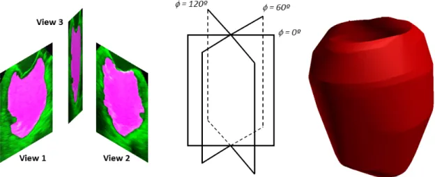
2.2.3 3D LV Volume Reconstruction . . . 64
2.3 Evaluation and Results . . . 64
2.3.1 Automatic Direct Frame LV Segmentation Evaluation . . . 66
2.3.2 Registration-based Blood-pool Propagation Evaluation . . . . 66
2.3.3 3D Volume Reconstruction Evaluation . . . 67
2.4 Discussion . . . 68
2.5 Summary and Future Work . . . 70
Cine Cardiac MRI 72
3.1 Introduction . . . 73
3.2 Methodology . . . 74
3.2.1 Data Preprocessing . . . 74
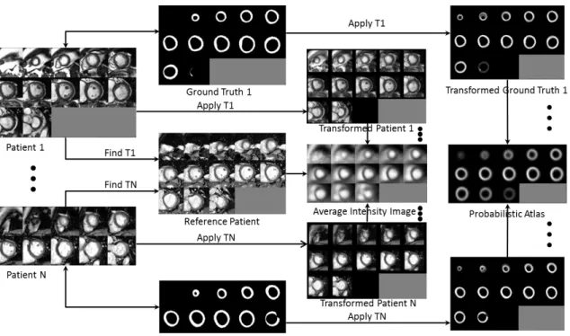
3.2.2 Atlas Generation . . . 76
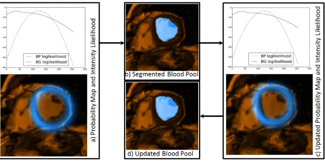
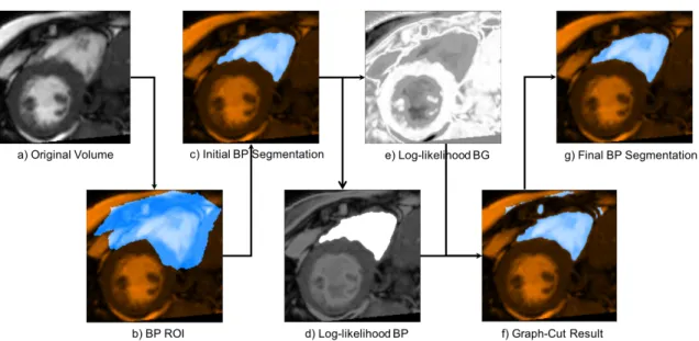
3.2.3 LV Blood Pool Segmentation using Iterative Graph Cuts . . . 76
3.2.3.1 Intensity Distribution Model: . . . 76
3.2.3.2 Blood Pool/Background Probabilistic Map: . . . 77
3.2.3.3 Graph-Cut Segmentation: . . . 78
3.2.3.4 Myocardial Probability Map Refinement . . . 79
3.2.3.5 Iterative Refinement: . . . 79
3.2.4 Myocardium Segmentation . . . 80
3.2.4.1 Intensity Distribution Model: . . . 81
3.2.4.2 Distance from the Endocardial Border: . . . 81
3.2.4.3 Graph-Cut Segmentation: . . . 82
3.3 Results . . . 82
3.4 Discussion, Conclusion, and Future Work . . . 84
4 Probabilistic Atlas Prior based Graph Cut Segmentation: Applica-tion and ValidaApplica-tion on Right Ventricle Slice-wise SegmentaApplica-tion from Cine Cardiac MRI 88 4.1 Introduction . . . 89
4.2 Methods . . . 90
4.2.1 Data Preprocessing . . . 90
4.2.2 Atlas Generation . . . 90
4.2.3 RV Blood Pool Segmentation using Iterative Graph Cuts . . . 91
4.2.3.1 Blood Pool Probabilistic Map: . . . 91
4.2.3.2 Blood Pool Initialization: . . . 92
4.2.3.3 Intensity Distribution Model: . . . 92
4.2.3.4 Graph-Cut Segmentation: . . . 93
4.2.3.5 Blood Pool Probability Map Refinement: . . . 95
4.2.3.6 Iterative Refinement: . . . 95
4.3 Results . . . 95
4.4 Discussion . . . 100
4.5 Conclusion and Future Work . . . 101
5 Towards Deep Learning Techniques for Cardiac Cine MRI Slice Mis-alignment Correction and 3D Hybrid Left Ventricle Segmentation 105 5.1 Introduction . . . 106
5.2 Methodology . . . 107
5.2.2 Data Preparation and Augmentation . . . 108
5.2.3 CNN Architecture for LV Center Regression . . . 108
5.2.4 Slice-misalignment Correction . . . 109
5.2.5 LV Blood-pool Segmentation . . . 110
5.2.5.1 Atlas Generation . . . 110
5.2.5.2 Blood-pool Label Transfer . . . 111
5.2.5.3 Graph-cut Segmentation . . . 111
5.2.5.4 Segmentation Refinement using Intersection-over-Union115 5.2.5.5 Iterative Segmentation Refinement . . . 117
5.2.5.6 Segmentation Refinement using Stochastic Outlier Se-lection . . . 118
5.3 Implementation Details . . . 119
5.4 Results . . . 121
5.5 Discussion, Conclusion, and Future Work . . . 124
6 Left Ventricle Segmentation and Quantification from Cardiac Cine MR Images via Multi-task Learning 128 6.1 Introduction . . . 129
6.2 Methodology . . . 129
6.2.1 Data Preprocessing and Augmentation . . . 130
6.2.2 MTL using Uncertainty-based Loss Weighting . . . 130
6.2.3 Network Architecture . . . 132
6.3 Results . . . 134
6.4 Discussion, Conclusion, and Future Work . . . 140
7 A Distance Map Regularized CNN for Cardiac Cine MR Image Seg-mentation 144 7.1 Introduction . . . 145
7.2 Methods and Materials . . . 148
7.2.1 CNN for Semantic Image Segmentation . . . 148
7.2.2 Distance Map Regularization Network . . . 151
7.2.3 MTL using Uncertainty-based Loss Weighting . . . 153
7.2.4 Clinical Datasets . . . 153
7.2.4.1 Left Ventricle Segmentation Challenge (LVSC) . . . 153
7.2.4.2 Automated Cardiac Diagnosis Challenge (ACDC) . . 154
7.2.5 Data Preprocessing and Augmentation . . . 154
7.2.6 Network Training and Testing Details . . . 155
7.2.7 Evaluation Metrics . . . 156
7.3 Results . . . 156
7.3.1 Segmentation and Clinical Indices Evaluation . . . 156
7.4 Discussion . . . 171 7.5 Conclusion . . . 175
8 Discussion, Conclusion, and Future Work 182
8.1 The Big Picture . . . 182 8.2 Summary and Contributions . . . 185 8.3 Future Directions . . . 188
2.1 LV blood-pool area comparison between proposed vs manual segmen-tation . . . 65 2.2 LV blood-pool segmentation evaluation against manual annotation:
Dice, Hausdorff, mean absolute distance, endocardial TRE . . . 66 2.3 LV blood-pool volume and ejection fraction comparison between
pro-posed vs manual segmentation . . . 67 3.1 LV myocardium segmentation evaluated against expert manual
anno-tation: Dice, Jaccard, Sensitivity, Specificity, PPV, and NPV . . . 83 3.2 LV myocardium segmentation results compared against other
pub-lished methods . . . 83 4.1 RV blood-pool segmentation evaluated against the expert manual
seg-mentation: Dice, Jaccard, mean absolute distance, and Hausdorff dis-tance . . . 96 4.2 RV blood-pool segmentation evaluated against the expert manual
seg-mentation compared against other published methods . . . 97 4.3 Comparison of computed end-diastole RV blood-pool volume against
manual estimate . . . 98 5.1 Slice misalignment errors before and after correction . . . 121 5.2 End-diastole LV blood-pool segmentation compared against manual
delineation: Jaccard, Dice, Hausdorff distance and mean surface distance122 5.3 End-diastole LV blood-pool segmentation compared against other
pub-lished methods . . . 123 6.1 Evaluation of segmentation results obtained from baseline and
pro-posed method against gold-standard segmentation . . . 135 6.2 Comparison of the Mean absolute difference between the gold-standard
myocardium area and the area obtained from three different methods 137
other published methods . . . 138 7.1 Model complexity, training and testing time . . . 156 7.2 Evaluation of the average segmentation results on ACDC dataset . . 160 7.3 Comparison of the segmentation results obtained from the DMR-UNet
model against the top three ACDC challenge participants . . . 162 7.4 Evaluation of the segmentation results on LVSC dataset . . . 163 7.5 Comparison of the LV myocardium segmentation results on the LVSC
validation set against the consensus segmentation . . . 164 7.6 Cross-dataset segmentation evaluation for LV myocardium segmentation166 7.7 Evaluation of the segmentation results on ACDC dataset obtained from
different weighting schemes of the categorical cross-entropy loss . . . 170
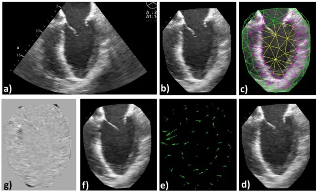
2.1 LV segmentation workflow . . . 59
2.2 Frame-to-frame image registration workflow . . . 62
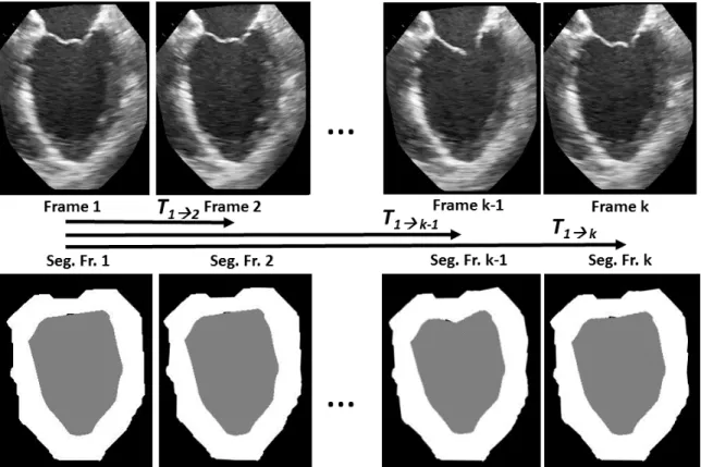
2.3 Frame-to-frame segmentation propagation via registration . . . 63
2.4 3D LV reconstruction . . . 64
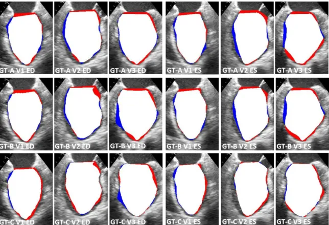
2.5 Expert manual segmentation of the LV . . . 65
2.6 Qualitative evaluation of the LV blood-pool segmentation . . . 68
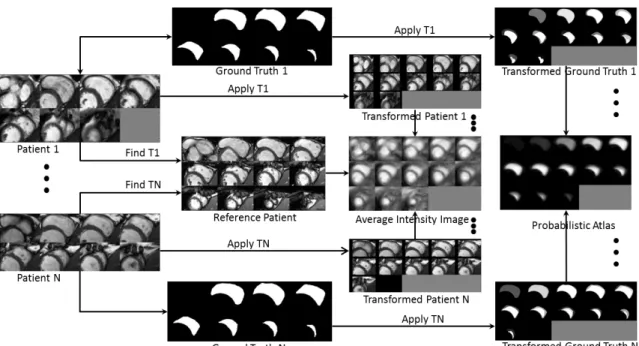
3.1 LV probabilistic atlas generation . . . 75
3.2 LV blood-pool segmentation workflow . . . 77
3.3 Iterative LV blood-pool segmentation refinement . . . 80
3.4 LV myocardium segmentation workflow . . . 81
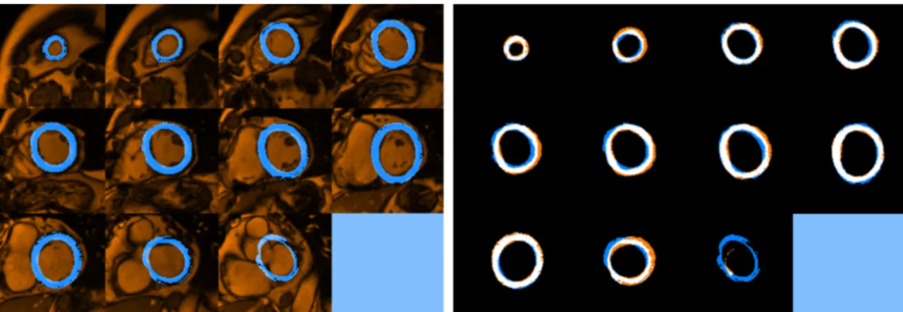
3.5 Qualitative evaluation of the LV myocardium segmentation . . . 84
4.1 RV probabilistic atlas generation . . . 91
4.2 RV blood-pool segmentation workflow . . . 92
4.3 Iterative refinement of the RV blood-pool segmentation . . . 94
4.4 Qualitative evaluation of the RV blood-pool segmentation . . . 96
4.5 3D visualization of the RV blood-pool segmentation . . . 98
4.6 Signed distance error visualized on the RV blood-pool surface . . . . 99
4.7 Quantitative evaluation of computed blood-pool volume against man-ual estimate . . . 99
5.1 CNN architecture for regression of the LV center . . . 109
5.2 3D LV models before and after slice misalignment correction . . . 110
5.3 Visualization of different stages in LV blood-pool segmentation . . . . 112
5.4 Histogram for misalignment errors before and after the correction . . 121
5.5 Boxplot for misalignment errors before and after the correction . . . . 122
5.6 Qualitative evaluation of the LV blood-pool segmentation . . . 123
6.1 Multi-task network architecture for myocardium segmentation and its area estimation . . . 133
6.2 Bar-plots for segmentation evaluation . . . 136
6.4 Box-plots and Bar-plots for the mean absolute difference between the gold-standard and myocardium area obtained from three different meth-ods . . . 139 7.1 Baseline FCN architectures and their simplified block representation . 149 7.2 Distance map regularizer added to the bottleneck layer . . . 151 7.3 Segmentation results for LV pool, LV myocardium, and RV
blood-pool . . . 157 7.4 Ground-truth and automatic segmentation obtained from all trained
models for a test patient . . . 158 7.5 Visualization of (a) the segmentation obtained by thresholding the
pre-dicted distance map and (b) absolute error between the ground-truth and predicted distance maps for all chambers. . . 159 7.6 Average Dice coefficient on apical, basal, and mid slices for ACDC
dataset . . . 161 7.7 Quantitative segmentation results on ACDC dataset divided according
to the five sub-groups . . . 162 7.8 Feature maps visualized for the UNet and DMR-UNet model . . . 167 7.9 Training and test curves, and the learned weights for cross-entropy and
mean absolute difference losses, for ACDC and LVSC dataset across five-fold cross-validation . . . 169 7.10 Average Dice coefficient for Learned vs Fixed equal weighting . . . . 172 7.11 Average Dice coefficient for a range of distance map thresholds . . . . 173 7.12 Weights distribution before and after distance map regularization . . 174
2D Two-Dimensional
3D Three-Dimensional
4D Four-Dimensional
AAM Active Appearance Model
ACDC Automated Cardiac Diagnosis Challenge
API Application Programming Interface
ASM Active Shape Model
BOLD Blood Oxygen Level Dependent
BP Blood Pool
BG Background
CNN Convolutional Neural Network
CPU Central Processing Unit
CRF Conditional Random Field
CT Computed Tomography
CTA Computed Tomography Angiography
DCM Dilated Cardiomyopathy
DFCN Densely Connected Fully Convolutional Network DICOM Digital Imaging and Communications in Medicine
DM Dice Metric
DM Distance Map
DMR Distance Map Regularized
DMTRL Deep Multitask Relationship Learning Network
ECG Electrocardiogram
EF Ejection Fraction
EM Expectation-Maximization
ES End-systole
ESV End-systolic Volume
FA Fully-Automatic
FCN Fully Convolutional Network
FIMH Function Imaging and Modeling of the Heart
FOV Field of View
GMM Gaussian Mixture Model
GPU Graphics Processing Unit
GVF Gradient Vector Flow
HCM Hypertrophic Cardiomyopathy
HD Hausdorff Distance
HU Hounsfield Unit
ICE Intracardiac Echocardiography
ICM Iterated Conditional Mode
IoU Intersection-over-Union
IPP Image Orientation Patient
ITK Insight Segmentation and Registration Toolkit
JM Jaccard Metric
KHz Kilohertz
LA Long-Axis
LoA Limits of Agreement
LoG Laplacian of Gaussian
LRW Lazy Random Walk
LV Left Ventricle
LVSC Left Ventricle Segmentation Challenge
MAD Mean Absolute Distance
MHz Megahertz
MICCAI Medical Image Computing and Computer Assisted Intervention
MINF Myocardial Infarction
MR Magnetic Resonance
MRF Markov Random Field
MRI Magnetic Resonance Imaging
MSD Mean Squared Difference
MSD Mean Surface Distance
MST Minimal Spanning Tree
MTL Multi-Task Learning
MTN Multi-Task Network
NCC Normalized Cross-Correlation
NMR Nuclear Magnetic Resonance
NPV Negative Predictive Value
PC Personal Computer
PET Positron Emission Tomography
PPV Positive Predictive Value
RAM Random Access Memory
ReLU Rectified Linear Unit
RF Radio Frequency
ROI Region of Interest
RV Right Ventricle
RVSC Right Ventricle Segmentation Challenge
SA Simulated Annealing
SA Semi-Automatic
SA Short-Axis
SD Standard Deviation
SOS Stochastic Outlier Selection
SSFP Steady State Free Precision
STACOM Statistical Atlases and Computational Models of the Heart STAPLE Simultaneous Truth and Performance Level Estimation
TE Echo Time
TEE Transesophageal Echocardiogram
TR Repetation Time
TRE Target Registration Error
TTE Transthoracic Echocardiogram
US Ultrasound
WHO World Health Organization
Introduction, Background, and
Thesis Overview
The goal of this chapter is to provide the reader with an overview of the clinical background for the proposed work, along with a brief and timely review of the literature on medical image segmentation, while identifying current clinical challenges.
1.1
Medical Imaging
Medical imaging is a noninvasive technique of creating the visual representation of the structure and function of interior organs of a body. When a body is exposed to some form of energy that can penetrate through and interact with the tissues, the detected signal containing information about the anatomical interaction can be used to construct an image [1]. Hence, medical imaging can be interpreted as a solution to a mathematical inverse problem, where the properties of tissue (cause) is inferred from the observed energy signal (effect).
Visible light energy is used mostly outside the radiology department in light mi-croscopy [2], endoscopy [3], and optical coherence tomography [4], due to its limited ability to penetrate tissues at depth; whereas the electromagnetic spectrum outside of the visible regime is typically used in diagnostic radiology. Depending on the type of energy and the acquisition technology used, different modalities of medical
images can be acquired. Some common imaging modalities routinely used in clin-ical radiology are x-rays, computed tomography (CT), magnetic resonance imaging (MRI), ultrasound (US), and nuclear medicine — single photon emission computed tomography (SPECT), positron emission tomography (PET) [5–8]. There is no single best imaging modality; rather, different imaging modalities are suitable for different applications and provide complementary information about the patient.
1.1.1
X-Ray Imaging
X-ray is the first imaging modality discovered in 1895 by German physicist Conrad Roentgen, who received the Nobel Prize in 1901 as he demonstrated its diagnostic abilities for imaging human body. Diagnostic X-rays have a wavelength between 0.01nm and 0.1nm (corresponding to 123 keV to 12.3 keV energy range) with reason-able attenuation to discriminate bone, soft tissue, and air. Since X-ray photons carry enough energy to ionize atoms and disrupt molecular bonds, it is an ionizing modality, and is harmful to living tissue with increased risk of radiation-induced cancer [9].
During imaging, the X-rays are transmitted through the body and collected on a film or an array of detectors. Since the X-rays are attenuated more by bones than soft tissues or air, the collected two-dimensional (2D) attenuation map serves as an image with excellent spatial resolution. Despite its harmful effects, X-ray is extensively used in the diagnosis of broken bones, lung cancer, breast cancer, etc. when the risk is greatly out-weighted by the benefits of the examination.
1.1.2
Computed Tomography Imaging
Two-dimensional images produced by X-ray are not adequate for many diagnostic applications requiring three-dimensional (3D) quantitative and qualitative informa-tion about the anatomical structures. This led to the development of Computed Tomography (CT); tomography referring to a picture (graph) of a slice (tomo). The X-ray source and detector are mounted on a gantry that rotates around the pa-tient capturing 2D projections from multiple angular view-points, which are then reconstructed into a 3D axial slice through the patient via back-projection algorithm
[7, 10, 11]. The patient lying on a movable bed is moved axially to acquire multiple axial slices that are stacked together to produce a 3D CT image.
The reconstructed image represents the linear attenuation coefficient map of the scanned object, which is converted to the standard Hounsfield unit (HU) correspond-ing to the actual intensity values of the CT image.
CT number = µ−µwater
µwater
×1000 (1.1)
In a CT image, the intensity value for water is 0 HU, air is -1000 HU, and soft tissue, bones have values from several hundred to several thousand HU, respectively.
The capability of modern helical and multislice CT scanners to produce very high quality (less than 0.5mm isotropic resolution) full body scans in less than 1 minute acquisition time has established it as the most widespread diagnostic imaging modality. CT scans are routinely used in clinic for head/full-body scan for diagnosis of accident injuries, dental planning, detection of lung nodules, diagnosis of lung emphysema, etc. Similarly, contrast enhanced CT is used for perfusion analysis of brain, liver, and tumors, as well as analysis of vessels for stenoses and aneurysms. Furthermore, the fast acquisition time of CT is suitable for cardiac imaging, hence, is used for quantification of coronary artery calcification and examining the dynamic motion of the heart muscles to detect abnormalities.
As CT scan involves multiple x-ray acquisitions, the patient is exposed to high ionizing radiation, increasing the risk of cancer [12]. Hence, since the development of the first clinical CT scanner in early 1970s, the field is mostly driven by the motivation of reducing the acquisition time and lowering the radiation dose, while maintaining the quality of images.
1.1.3
Magnetic Resonance Imaging
Magnetic Resonance Imaging (MRI) is a tomographic imaging technique that produces 3D images of the human body based on the Nuclear Magnetic Resonance (NMR) phenomenon. As the human body is mostly composed of fat and water, con-sisting of hydrogen atoms, the NMR signals from the nucleus of these hydrogen atoms
can be recorded by applying an external magnetic field gradient and appropriate ra-dio frequency (RF) pulse sequence to record k-space data, which is inverse fourier transformed to construct an MRI image [13, 14].
The density of hydrogen atoms for fat, muscle, and other tissues are different, hence rendering MRI as a powerful soft-tissue contrast imaging method. It is a versatile modality, as different tissues can be highlighted in the images by changing the acqusition parameters such as RF pulse sequence, repetation time (T R), and echo time (T E). Similarly, the image slices can be acquired in any direction by changing the external magnetic field gradients. Furthermore, with the faster acquisition of images by exploiting the mathematical properties of the k-space, parallel acquisition techniques, and the advent of new RF pulse sequences, it is possible to perform MRI angiography, diffusion imaging, as well as functional imaging based on the blood oxygen level dependent (BOLD) response.
MRI has been a popular modality for medical diagnosis due to the lack of ionizing radiation and high contrast sensitivity to soft tissues. However, it is limited by slower acquisition speed, high equipment and siting cost, operational complexity, significant imaging artifacts, and MR safety concerns.
MRI is the preferred cardiac imaging modality due to its capability of tissue characterization. Specifically, the steady state free precision (SSFP) pulse sequence [15], which reduces the acquisition time while maintaining a good signal-to-noise ratio as well as good blood-myocardium contrast, is coupled with electrocardiogram (ECG) gating to produce movie of a heart slice throughout the cardiac cycle, known as cine MRI acquisition. The short-axis cine MR slices covering the whole heart are stacked together to generate a pseudo four-dimensional (4D) volume, which can be used to perform quantitative analysis of cardiac indices [16]. However, since very few slices are acquired due to higher acquisition time, and the slices might be misaligned due to breathing/patient-motion, 3D analysis of cine MR images is challenging. In this thesis, we use open-source cine MRI datasets for cardiac image segmentation.
1.1.4
Ultrasound Imaging
Sound waves with frequencies above 20 kilohertz (KHz), the upper audible limit of human hearing, are termed as ultrasound (US). US imaging devices constitute of piezoelectric crystal-based transducer that produces the ultrasound beam (typically 1-15 megahertz (MHz)) as well as receive the returned echo from the tissue [17].
A-modeimaging is the simplest form of US imaging where the transducer transmits US pulses through the patient body such that the time and amplitude of the received echos provide the location information and the tissue structures and interfaces along the path, respectively. Hence, a vector image with spatial dimension representing the location and the intensity representing the amplitude of received echo is generated.
M-mode images are formed by arranging A-mode vector images, along a fixed US beam at different time instances, in columns of a 2D matrix. These images are useful to analyze moving objects inside the body.
B-Mode images are constructed by pivoting the transducer at a point about an axis acquiring several A-mode vector images, along a V-shaped imaging region, and combining them into a 2D matrix. This is the most commonly used imaging mode.
Real-time 3D US imaging is now possible using 2D array of transducer with beam-forming electronic in the transducer handle. Similarly, doppler US can be used to measure the flow velocities based on the shift of frequency in an ultrasound wave due to blood/liquid flow. Furthermore, gas-filled encapsulated microbubbles can be used as contrast agents to enhance the echo amplitudes and hence the image contrast.
Due to low-cost, portability, real-time, and ionizing-radiation-free acquisition, US is used in various clinical applications such as breast, cardiac, gynecologic, obstetrics, pediatrics, and vascular imaging. However, the images suffer from various artifacts such as speckle noise due to the random alignment of sound waves reflected on mi-croscopic tissue inhomogeneties, shadows casted behind a strong reflecting object,
multiple reflections between two strong reflectors displayed as multiple echos, and
mirroring when an object is placed between the transducer and a strongly reflecting
layer [6].
functions, blood-flow measurement using doppler imaging, and myocardial deforma-tion evaluadeforma-tion using strain imaging [18]. Transthoracic echocardiogram (TTE) is the most common non-invasive assessment, where the heart is imaged by placing the US probe on the chest or abdomen of the patient. However, the quality of acquired image is low due to the signal attenuation by layer of fat and muscle on the US path. Transesophageal echocardiography (TEE) produces better images by passing a specialized probe containing an ultrasound transducer at its tip into the patient’s esophagus and imaging the heart from close. Similarly, Intracardiac echocardiography (ICE) performed through a venous or arterial sheath is able to produce high resolu-tion images from within the heart without the need for general anesthesia. However, it has limited field-of-view and high associated cost because of single-use catheters. Hence, TEE is generally the preferred US protocol in the clinic. In this thesis, we use the multi-plane TEE image sequences for LV segmentation and 3D reconstruction.
1.1.5
Nuclear Medicine Imaging
Nuclear medicine [19] refers to a branch of radiology where a patient is injected with substances containing radioactive isotope such that the x- and/or gamma rays emitted during radioactive decay detected by a radiation detector is used to make projection images. The acquired multiple projection images are back projected to reconstruct a tomographic slice, similar to CT imaging. It is a functional imaging modality since it provides physiological information of imaged organs, as the emis-sivity of a healthy tissue is different from a diseased one. Hence, the nuclear images are usually coupled with the structural CT images to analyze both the structure and function of organs.
Most popular nuclear medicine imaging techniques are SPECT and PET. In SPECT, the tomographic images are reconstructed from the x- or gamma-ray emis-sions from the patient detected by a nuclear camera at multiple angles around the patient. In PET, the positron (e+) emitted during the decay of an isotope combines
with an electron (e−) to produce an annihilation radiation emitting two photons in opposite directions; the detected photon pairs give information about a straight line
along which the annihilation event took place and can be used to compute the 3D distribution of the PET agent and hence generate a tomographic emission image. PET is more sensitive to small physiological changes in tissues than SPECT at an expense of higher imaging cost.
Typically the functional images acquired from SPECT and PET are combined with structural CT images; SPECT-CT and PET-CT imaging are often used in car-diology, oncology, neurology, and imaging of infection and inflammation.
1.2
Image Segmentation
Image segmentation refers to the grouping of pixels/voxels in an image based on common properties such as intensity, color, texture, and location [20, 21]. The segmentation task assigns a label to each pixel/voxel in an image based on its features. Clinicians often require to delineate an organ, tumor, vessels, etc from the acquired X-ray, MRI, CT, or US images for diagnostics, planning and guidance. Although the manual delineation is referred to as the gold-standard, it is time intensive (specially for 3D/4D images), and is prone to intra- and inter-observer variability. Hence, it is often desirable to perform semi-/fully-automatic segmentation that can be manually adjusted if desired.
Based on the amount of prior knowledge used, image segmentation algorithms can be broadly classified into (i) No prior, (ii) Weak prior, (iii) Strong prior, and (iv) Machine learning based methods.
1.2.1
No Prior Based Algorithms
These are the simplest kind of segmentation algorithms that do not use any prior information about the shape/geometry of the object and rely only on the pixel/voxel intensity information.
1.2.1.1 Thresholding
Thresholding algorithms determine the intensity thresholds, T1 and T2, based
on the intensities of the input image, I(x), such that the foreground/background separated binary image, S(x), can be obtained as:
S(x) = 1 if T1 ≤I(x)≤T2 0 otherwise (1.2)
Otsu’s method [22] provides an optimal global threshold that minimizes the intra-class intensity variance while maximizing the inter-class intensity variance for an image with bi-modal histogram. Multi-level thresholding can be used to delineate multiple foreground objects from the background. Similarly, adaptive thresholding based on the local image statistics is preferred when the image statistics vary significantly in different image regions, possibly due to imaging artifacts.
1.2.1.2 Edge Detection and Linking
Edges can be detected from an image using a discrete approximation of the deriva-tive operator along each spatial dimension, based on the intensity differences between the neighboring pixels. The first order derivative operator is approximated by sev-eral discrete filters such as Roberts, Prewitt, and Sobel. Similarly, the second order derivative operator is approximated by a discrete Laplacian filter.
Due to the high sensitivity of derivative operator to noise, usually the image is smoothed by a Gaussian filter before edge detection. Laplacian of Gaussian (L0G) filtering can produce fine edges based on zero-crossings. The obtained discontinuous edges can be linked based on the proximity, edge strength, and edge direction, to generate a continuous boundary. Canny edge detection [23] algorithm uses a multi-stage pipeline to produce fine boundaries of the objects in an image. Similarly, Hough transform [24] can be used to detect the geometric objects such as line, circle, and ellipse from the edges.
1.2.1.3 Region Growing
Region growing algorithm groups pixels or subregions into a larger region based on a predefined criteria. The algorithm requires manual/automatic ”seed” points, such that the neighboring pixels with features (intensity, texture) similar to the seed are appended to grow the region. Region growing stops when no more neighboring pixels satisfy the inclusion criteria, resulting in segmented image with multiple foreground regions.
1.2.1.4 Morphological Watershed
In the morphological watershed algorithm [25], the images are interpreted as a topographical map with image intensity representing an additional dimension. For example, a 2D image can be viewed as a 3D topographical map with the third di-mension representing the pixel intensity. The pixels with minimum intensity within a topographical region are termed as regional minimum, which can be obtained via image smoothing followed by local/global thresholding.
The basic principle of the watershed algorithm is to punch a hole in each regional minimum and flood the entire topography by letting water rise through the holes at a uniform rate. When the rising water in distinct catchment basins is about to merge, a dam is built to prevent the merging. At the end of flooding, when only the top of the dams are visible above the water line, the dam boundaries dividing the watersheds corresponds to the continuous boundary between the segmented regions.
1.2.2
Weak Prior Based Algorithms
These algorithms pose segmentation as a global energy minimization problem in an image, while imposing weak constraints such as piecewise continuity of segmented regions, and smooth curvature of the segmented boundary. The use of global image context and weak prior knowledge generates superior segmentation results compared to the no prior based algorithms, at an expense of higher computation cost.
1.2.2.1 Deformable Models
These models pose the segmentation problem as an energy minimization problem in variational framework.
Active Contours or Snakes
Active contours are the parameterized spline curves that are evolved based on the internal spline energy and the external image forces, to lock onto nearby edges of the objects to be segmented in an image [26]. The snake is represented parametrically by v(s) = (x(s), y(s)), where 0≤s≤1, with the total energy functional represented as the sum of internal and external energy functionals:
Esnake∗ =
Z 1
0
Eint(v(s)) +Eext(v(s)) (1.3) Where the internal spline energy can be written as:
Eint(v(s)) = 1 2 α(s)|vs(s)| 2+β(s)|v ss(s)|2 (1.4) The first- and second-order terms control the amount of stretch and the amount of curvature in the snake and are weighted byα(s) andβ(s), respectively. The external energy term, Eext(v(s)), is formulated as the weighted combination of the image in-tensity, negative image gradient magnitude, and the curvature of level contours in the original paper [26]. Starting with an initial curve selected manually/automatically, the Euler equations corresponding to the energy functional of equation1.3are solved iteratively until convergence to obtain the stationary point, yielding the final segmen-tation result.
Due to the internal spline energy forces, the snake would collapse into a point or a line (depending on if the curve is closed or open, respectively) if placed in a region with uniform intensity. Cohen [27] proposed a modification to the external energy to include a ”balloon” (pressure) force acting outward (or inward) in the normal direction of the curve, allowing the curve to inflate (or deflate) and hence avoid the collapse. The direction of the pressure force could be changed depending on the requirement of expanding/shrinking the snake.
The snake formulation still suffers from two major limitations: the curve has to be initialized fairly close to the final solution due to the limited capture range of the image gradient force, and the convergence to boundary concavities is poor. These limitations were solved by the introduction of gradient vector flow (GVF) [28] as the external energy term in the snake formulation. The GVF, computed as a diffusion of the gradient vectors of a gray-level or binary edge map derived form the image, increases the capture range of snakes as well as help them move into the boundary concavities. Several modifications for the external energy term have been proposed in the literature to further improve the performance of the snakes.
Level Sets
The level set framework [29] can handle topology changes during contour evolu-tion, process multiple contours simultaneously, and allow cusps and corners, which is not possible with the parametric representation of curve in active contour model. The interface, dΩ, (a curve in 2D or a surface in 3D) is represented implicitly by zero-contour of a higher dimension Lipschitz continuous function, φ, as dΩ(t) =
{x|φ(t,x) = 0}. In practice the signed distance function is chosen as the level-set function: φ(x) = −d forx∈Ω− +d for x∈Ω+ 0 for x∈dΩ (1.5)
where d is the Euclidian distance to dΩ. The evolution equation of the level set function can be written as:
∂φ
∂t +F|∇φ|= 0, φ(0,x) =φ0(x) (1.6)
where, the functionF is called the speed function and the set {x|φ0(x= 0)} defines
the initial interface. The level set function can be used to compute the normal to the interface n and the interface’s mean curvature κ as:
For the motion by mean curvature, the speed function can be selected as F = κ. Similarly, the speed function can be modified by a monotonously decreasing function of the image gradient magnitude, g(|∇I0|), to stop the level set evolution on the
desired boundaries [30].
Since the level set function does not retain its signed distance function properties as it evolves in time through equation 1.6, it needs to be reinitialized periodically after every few iterations [31]. The reinitialization might move the level set incorrectly, while increasing the computation cost. Hence, Li et al.[32] proposed a variational framework that penalized the movement of level set away form the signed distance function and did not require reinitialization during the evolution.
Caselles et al.[33] formulated the classical energy-based active contour model (1.2.2.1) as a problem of finding a geodesic curve in a Riemannian space derived from the image content; equivalent to finding a curve of minimal weighted length in certain framework. This level set based geodesic active contour framework exploited the connection between the classical energy-based model and the intrinsic level set model. The geodesic formulation introduced a new term that further attracted the deforming curve to the boundary and hence improved the convergence, while also reducing the number of hyper-parameters.
The early active contour and level set formulations used image gradients as the external force to determine the object boundaries, hence, they struggled with noisy images and failed to segment objects with weak/smooth boundaries. Chan and Vese [34] proposed a region-based segmentation model based on the minimization of Mumford-Shah functional [35] for segmentation. The corresponding energy mini-mization problem is equivalent to the minimal partition problem, and is solved via level set evolution using finite difference approximation. Since the method does not depend on image gradients, the energy landscape is smoother, resulting in better con-vergence, even with poor initializations. Most recent level-set segmentation methods employ both gradient- and region-based external energy terms to obtain more robust segmentation results.
1.2.2.2 Graph Theoretical Models
Graph theoretical models represent an image as a discrete graph and pose the segmentation as a combinatorial graph partitioning problem. For a graphG= (V, E),
V ={v1, ..., vn}is a set of vertices representing the image elements (pixels/voxels/super-pixels), and E is a set of edges connecting pairs of neighboring vertices. Each edge (vi, vj)∈ E is weighted by a weight w(vi, vj) based on the properties of the two ver-tices connected by the edge, hence introducing weak constraint into the framework. The image segmentation problem is formulated as a partitioning of the graph Ginto mutually exclusive connected sub-graphs Gs = (Vs, Es), where Vs ⊆V, Es⊆ E, and
s = {1,2, ..., k}, such that {Gi∩Gj = φ : i, j ∈ {1,2, ...k}, i 6= j} and G = k
S
s=1
Gs. Where the properties of vertices (intensity, texture, color, etc) within a sub-graph should be similar, while that between different sub-graphs should be dissimilar.
The degree of dissimilarity between the subgraphs can be computed as a graph cut. A cut partitions the graph into disjoint connected sub-graphsGa andGb and its value is defined as:
cut(Ga, Gb) =
X
va∈Ga,vb∈Gb
w(va, vb) (1.7)
which is the sum of weights of all the edges connecting Ga and Gb. Hence, image segmentation is equivalent to finding the optimal cut in the graph. A comprehensive survey of graph theoritical models for image segmentation can be found in [36]
Minimal spanning tree based methods
A spanning tree is an acyclic sub-graph (tree) including all vertices of the con-nected graph, G, but with a single path between any two vertices. Out of multiple spanning trees in a graph, the minimal spanning tree (MST) is the one with small-est edge weights; it can be computed using several algorithms [37–39]. For example, Kruskal’s algorithm [37] list all of the edges in ascending order and adds edge con-nected to the MST with smallest weight, without generating any cycles. Next, if we consider a binary image segmentation problem, the task is to find and remove a single edge dividing the MST into two connected sub-graphs of descent sizes, such that the
intra-class variance is minimized while the inter-class variance is maximized. In case of multi-class labeling, multiple edges can be removed to obtain multiple connected sub-graphs representing segmented regions. MST based image segmentation can be found in several papers [40–42]
Shortest path based methods
Shortest path based methods obtain the segmentation boundary by finding the shortest path between vertices in a weighted graph. Most of these methods rely on manual input points to guide the segmentation boundary to the desired location.
Intelligent Scissors [43] framework allows objects in a digital image to be extracted
quickly and accurately using mouse gestures. An user starts tracing from a point and as s/he move the cursor closer to the boundary of the object, the live-wire boundary snaps to the object boundary. The live-wire boundary position is the shortest path from the previous boundary point to the current cursor location computed using optimal graph search (Dijkstra [44]) and dynamic programming in a 2D weighted graph, with edge weights defined as the weighted combination of Laplacian zero-crossing, gradient magnitude, and gradient direction. Similar algorithm based on the user interaction using mouse cursor has been proposed in [45]. Furthermore, 3D extensions of the shortest path based segmentation methods can be found in [46, 47]. Geodesic shortest path formulation computes the geodesic distance of each pixel to the labeled forground or background pixels and assigns a label to the pixel depending on the shortest geodesic path [48]. The geodesic paths are weighted according to the image contents.
Random walk based methods
Random walk based methods represent an image as a graph with edge weights proportional to the image gradients. An interactive multi-class segmentation of the image can be obtained based on the seed points provided by an user, such that the probability of a particular pixel assigned to classk is determined by the probability of a random walker starting at that pixel first reaching thekthseed point. Hence, for each
pixel a tuple ofk probabilities are computed corresponding tok-classes, and the final segmentation is obtained by assigning a pixel to the class with highest probability. Grady [49] presented an algorithm to compute random walk probabilities by solving a set of sparse linear systems, obtaining good segmentation results on synthetic and real images.
Shen et al.[50] proposed a lazy random walk (LRW) algorithm [51] for superpixel segmentation. Adding a self-loop over the graph vertex makes the random walk process lazy and help make full use of the global relationship between the pixel and all the seeds. A vertex with heavy self-loop is more likely to absorb its neighboring pixels than the one with light self-loop, which enables the vertex to absorb and capture both the weak boundary and texture information. Furthermore, since the LRW algorithm computes the commute time from seed-point to other pixels, as opposed to starting from the pixels to the seed-point in original random walk algorithm, it produces better probability maps, hence generating excellent superpixel results.
Several modifications of random walk algorithm (sometimes in conjunction with other methods) have been proposed for segmentation of various structures from med-ical images [52–54].
Graph cut based on Spectral Clustering
Spectral clustering is a dimensionality reduction technique which uses specturm (eigenvectors) of the graph similarity matrix for data clustering. It has an equvalent interpretation as a graph cut and can be applied for image segmentation.
The weighted adjacency matrix of the undirected graph, G = (V, E), is the symmetric n ×n matrix W = w(vi, vj). The degree of a vertex vi ∈ V is di =
Pn
j=1w(vi, vj). The degree matrix D is defined as the diagonal matrix with the
de-grees d1, ..., dn on the diagonal. The unnormalized graphLaplacian matrix is defined as L=D−W. If the partition of the graph is represented by x= [x1, ..., xn]T, such
the value of cut is given by: cut(Ga, Gb) = X va∈Ga,vb∈Gb w(va, vb) = 1 4 n X i,j=1 w(vi, vj)(xi−xj)2 = 1 2x TLx (1.8)
To avoid the trivial solution xi = 0, for all i, the following quadratic constraint is imposed: xTx=n. If we relax the requirement on xsuch that it can be real valued, the approximate solution to this constrained optimization problem can be obtained from the real eigenvector of the Laplacian matrix L with smallest eigenvalue.
(D−W)x=λx (1.9)
However, the smallest eigenvalue (λ1) is 0, yielding the noninteresting solution x =
[1, ...,1]. Therefore the second smallest eigenvalue (λ2) and the sign of the associated
eigenvector yields the optimal solution [55].
Since the minimum cut favors cutting small sets of isolated nodes in the graph, several modifications have been proposed to maintain resonably large clusters. Ratio cut [56] tries to optimize the following cost function:
RatioCut(Ga, Gb) = cut(Ga, Gb) |Ga| + cut(Ga, Gb) |Gb| (1.10) where,|.|represents the number of vertices in the graph. To obtain the ratio cut, the elements of eigenvector corresponding to λ2 are assigned to two clusters based on the
threshold that minimizes equation 1.10. Heuristically, the elements of the eigenvector,
xi ∈ IR, can be clustered into two groups using k-means clustering algorithm to determine the cluster of each vertex [57] .
Shi and Malik [58] introduced the normalized cut cost function to improve the balance between the cluster sizes after the graph cut:
N cut(Ga, Gb) =
cut(Ga, Gb)
vol(Ga) +
cut(Ga, Gb)
where, vol(Ga) =
P
i∈Ga,j∈Gw(vi, vj) is the total connection from vertices in Ga to
all vertices in the graph,vol(Gb) is defined similarly. The graph partition minimizing equation 1.11 can be obtained by solving the eigenvalue problem
(D−W)x=λDx (1.12)
The eigenvector corresponding to λ2 can be used to bipartition the graph. Each
sub-graph can be further partitioned recursively if necessary.
Several objective functions for graph partitioning have been proposed to maximize the inter-cluster similarity while minimizing the intra-cluster similarity [59, 60] to improve the clustering performance.
Graph cut on Markov random field models
Undirected graphical model with markov properties, also known as Markov ran-dom field (MRF), can encode the local spatial interaction between image pixels. MRF allows probabilistic interpretation of image segmentation, where an image,
x={x1, ...,xn}, has a random variable,xi, associated with each pixel. Eachxi needs to be assigned a label, L (foreground/background), during image segmentation.
The joint distribution of image label, x, can be written as a product of distri-butions of maximal cliques. Where a clique refers to a subset of nodes in a graph with an edge beween each node; maximal cliqueis a clique with maximum number of nodes. LetC be a clique andxC be the set of variables in that clique, then the joint distribution can be written as:
p(x) = 1
Z
Y
C
ψC(xC) (1.13)
whereψC(xC) is potential function of maximal clique C. Z is a normalizing constant called the partition function and is given by:
Z =X
x
Y
C
ψC(xC) (1.14)
which ensuresp(x) is a probability distribution. The potential functions are restricted to be non negative, ψC(xC)≥ 0, ensuring p(x) ≥0 (Hammersley and Clifford [61]).
The potential functions can be expressed as Gibbs Distribution [62, 63]:
ψC(xC) = exp{−E(xC)} (1.15)
whereE(xC) is theenergy functionof maximal cliquexC. Hence, the joint distribution defined as the product of clique potentials is equivalent to the Gibbs distribution of the total energy, which is the sum of energies of all maximal cliques. The maximum
a posteriori (MAP) estimate of the joint distribution yields optimum labeling of the
image, which is equivalent to the minimum energy configuration (equation 1.15). For a first order MRF, the total energy can be represented as:
E(f) = X {p,q}∈N Vp,q(fp, fq) + X p∈P Dp(fp), (1.16)
where the first term represents smoothness energy which enforces spatial smoothness between pixels in a set of interacting pairs, N, and the second term represents the data energy defined for each pixel based on its likelihood of being labeledfp.
Gemen and Geman [62, 63] first introduced the Bayesian image restoration us-ing MRF image model. They used the Gaussian distribution likelihood and isus-ing model prior to obtain the posterior distribution in the Bayesian framework. The MAP inference of the posterior distribution was performed by serial Gibbs sampling with simulated annealing (SA) [64] schedule. Besag [65] later proposed MAP esti-mation using Iterated Conditional Mode (ICM). ICM finds the mode for each node conditioned on all the neighbors based on the current estimate of variables, and syn-chronously updated the whole image repetadely until convergence. ICM can obtain a local maxima significantly faster with no guarantee of global convergence, while SA has a guaranteed global convergence provided a slow cooling schedule.
Greig et al.[66] discovered the minimum energy configuration of the MRF (corre-spondingly the MAP) is equivalent to the minimum cut in the graph. Hence, they computed the exact MAP estimate for a binary image restoration problem using the Ford-Fulkerson algorithm [67], which states that the minimum cut in a graph can be obtained from the maximum flow. Similarly, Wu and Leahy [68] performed data clustering using the maxflow-mincut approach on a specially constructed graph, and applied it on image segmentation.
The traditional SA and ICM optimization algorithms are slow because they allow small moves where only one pixel changes its label at a time. Boykov et al.[69] proposed two algorithms based on graph cuts that efficiently find a local minimum with respect to two types of large moves (large set of pixels changing labels) called expansion and swap moves. These algorithms have strong convergence guarantee within a known factor of the global minimum for two general classes of interaction penalty V: metric and semimetric. V is called a metric on the space of labels L if it satisfies:
V(α, β) = 0↔α=β, (1.17a)
V(α, β) =V(β, α)≥0, (1.17b)
V(α, β)≤V(α, γ) +V(γ, β) (1.17c) for any labels α, β, γ ∈ L. If V satisfies only (1.17a) and (1.17b), it is called a
semimetric1. Later, Kolmogorov and Zabih [70] characterized the energy functions
that can be minimized by graph cuts and also provided respective graph construction techniques. Recently, Kr¨ahenb¨uhl and Koltun [71] proposed an efficient approximate inference algorithm for fully connected conditional random field (CRF) model with pairwise edge potentials defined by a linear combination of Gaussian kernels.
1.2.3
Strong Prior Based Algorithms
These algorithms constraint the solution space based on the training examples and hence yield good segmentation results even with ill-defined or missing object boundaries. However, the imposed constraints are very strict, causing the algorithms to fail if the training set is not representative of the population.
1.2.3.1 Active shape and appearance models
The active shape model (ASM) learns the pattern of shape variability from the training set of correctly annotated images, such that, the result of a segmentation
algorithm can be constrained to plausible solutions [72]. ASM can be generated as follows:
• User marks multiple (n) corresponding landmarks, x = (x1, y1, ..., xn, yn)T ∈ IR2n, from N training examples.
• Align the training shapes by scaling, rotating, and translating, using Procrustes method [73].
• Compute the mean shape,x, using x= 1 N N X i=1 xi (1.18)
• Compute the 2n×2n covariance matrixS, using S = 1 N N X i=1 (xi−x)T(xi−x) (1.19)
• Perform eigen-decomposition of the covariance matrix,S, such that the columns of matrixP represent the eigenvectors, and the diagonal elements ofΛrepresent the eigenvalues (λi)
S =PΛPT (1.20)
• A shape in training set can now be approximated using the mean shape and the weighted sum of k eigenvectors with largest eigenvalues, represented by a 2n×k matrix Pk as:
x=x+Pkb (1.21)
with the corresponding weight vector b = (b1, ..., bk)T.
• New example shapes similar to those in training sets can now be generated by varying the parameters,bi’s, within suitable limits. The parameters are linearly independent, though there may be nonlinear dependencies still present. The variance of bk over training set is λk (kth eigenvalue), hence the suitable limits for plausible shapes lies within three standard deviations of the mean:
−3pλk≤bk≤3
p
The built ASM model can be used to constraint the evolution of the active contours (1.2.2.1) after each contour update. The residual deformation, dx, obtained after compensating for the translation, scale, and rotation of the model yields the parameter update, db, as:
db=PTkdx (1.23)
such that the model parameters can be updated as:
bt+1 ←bt+Wbdb (1.24)
where, Wb is a diagonal matrix of weights, which can be identity, or each weight can be proportional to the variance of the corresponding shape parameter over the training set, to allow rapid movement of parameters with higher variance. Further, the shape parameters, bi’s, can be restricted withing three standard deviations as in (1.22), to allow the evolved shape to be within a plausible range. Hence, the final segmentation, consistent with the training shapes, can be obtained via iterative updates upon convergence. The imposed shape constraint combined with the image information overcomes the segmentation challenges with missing object boundaries.
An Active Appearance Model (AAM) extends the ASM to include gray-level pearance of the object of interest. The built statistical model of the shape and ap-pearance is more robust, and can fit a test image even from poor starting estimates. Model fitting refers to finding the model parameters to minimize the sum of squared difference between the test image and the synthesized model. Since the gradient de-scent optimization for model fitting requires expensive gradient computation in each iteration, the original paper by Cootes et al.[74] learns the linear relationship between model parameter displacements and the residual errors (between a training image and a synthesized model example), such that, during model fitting, the current residual is used to predict the model parameter displacements leading to a better fit. To speed up the model fitting, several optimization algorithms have been proposed [75], includ-ing warpinclud-ing the model to the test image via piecewise affine transformation [76] usinclud-ing the inverse compositional image alignment [77] algorithm. A comprehensive review of statistical shape models for 3D medical image segmentation can be found in [78].
1.2.3.2 Atlas-based models
Atlas-based models solve the image segmentation problem via image registration. In the context of cardiac image segmentation, an atlas is a cardiac US/MR image coupled with the corresponding manual segmentation of the heart chambers. The optimum transform, registering the atlas image to a test image, can be applied to the atlas segmentation, to obtain the segmentation of the test image. Based on the num-ber of atlases used, atlas-based models can be divided into — single- , probabilistic-(average-), or multi-atlas based approach [79]. Atlas-based models have been exten-sively used for medical image segmentation [80, 81].
Single-atlas model
In this model, a single segmented image with good resolution and contrast is selected as an atlas. The atlas image is first registered to a test image via global similarity/affine transform and the alignment is further refined using a deformable transform. The obtained optimum transform (global+deformable) applied to the atlas label yields the test image segmentation.
Due to the large variability in test images, usually a single atlas in not sufficient to produce good results. Hence, multiple atlases can be registered to the test patient, such that, the segmentation obtained from the best atlas is selected. The best atlas can be chosen based on one of the two criteria — the atlas producing best similarity metric after global (and optionally deformable) registration, or the atlas requiring least deformation to register to the test patient.
Probabilistic atlas model
Multiple atlases can be registered to the same reference coordinate system, such that, the pixel-wise average intensity (after normalization) and labels provide the aver-age appearance of the anatomy and atlas, respectively. The probabilistic-atlas represents the probability of each pixel belonging to a specific label in the ref-erence coordinate system. Hence, the probabilistic-atlas for a specific group: gender, age, ethnicity etc. can be generated to better represent the variability in that group.
To segment a test image, the optimum transformation from the average appearance image (in the reference coordinate system) to the intensity normalized test image is obtained via registration, and hence the probabilistic-label is transferred. Further-more, the transferred label can be used as a prior probability and combined with a likelihood term in a Bayesian framework to obtain the maximum a posteriori (MAP) probability of each pixel belonging to a specific label. This framework is attractive as it is fast, requiring a single image registration step, while also incorporating the variability in the multiple training atlases.
Multi-atlas model
The multi-atlas model registers multiple atlases to the test image, hence, trans-ferring multiple labels. The label fusion step combines multiple labels to obtain the test image segmentation. Various label fusion strategies have been proposed in the literature [81, 82]. The simplest strategy is majority voting, where the label for each pixel is assigned according to the most frequent label obtained from multiple atlases. This strategy can be refined by assigning higher weights to the labels obtained form atlases with higher similarity to the test image (after registration). Furthermore, better segmentation performance can be obtained by weighting the atlases based on local image similarity. As the image registration is prone to errors, multi-atlas model is more robust compared to the single-/probabilistic-atlas models, at an expense of increased computational cost.
1.2.4
Machine Learning Based Algorithms
Machine learning algorithms recognize a pattern in the data using statistical tech-niques without being explicitly programmed. Supervised methods learn the mapping from the image intensity to the labels using the training image and corresponding segmentation, whereas the unsupervised methods try to find patterns in the image intensities to group similar pixels in the same class.
1.2.4.1 Unsupervised Methods
Unsupervised methods cluster the image pixels based on image features such as: intensity, color, and texture. Provided the number of clustersk, the k-means cluster-ing algorithm [83] assigns each pixel to a cluster by reduccluster-ing the within-class variance. Although attractive due to its simplicity, the k-means clustering algorithm assumes similar sized spherical clusters, and performs hard clustering (each data is assigned to a single class). The fuzzy c-means algorithm [84] extends k-means to produce soft clustering by providing the membership of each data point to multiple clusters. Sim-ilarly, the Gaussian mixture model (GMM) is a generalization of k-means algorithm, which can model non-spherical clusters, with soft assignment of data to multiple clusters. The Gaussian mixture model is estimated using the iterative Expectation-Maximization algorithm [85].
In contrast to the above mentioned clustering algorithms, the mean shift algorithm [86] does not require prior knowledge of the number of clusters, and does not constrain the shape of the clusters. The mean shift algorithm creates a window around each data point, finds the weighted mean of data within each window, shifts the window to the mean, and repeat until convergence. The windows that end up near the same peak/mode of the data density are merged and assigned to the same cluster. Hence, a robust cluster of data is generated at an expense of higher computational cost.
When the pixel location is used alongside the image features for unsupervised clustering, perceptually similar pixels can be grouped together to createsuper-pixels [87]. The obtained over-segmentation can be used as a preprocessing step for the subsequent image segmentation task.
1.2.4.2 Supervised Methods
Pixel-wise Classification
For pixel-wise classification, a set of features is extracted from each pixel, such as: image intensities in the fixed neighborhood patch, color information, Gabor filter output, image gradients, pixel location etc., and a discriminative model (Support Vector Machine [88], Random Forest [89] or Neural Network classifier [90]) is trained