Bayesian Imputation of Missing Covariates

(1)

(2)

Bayesian Imputation of Missing Covariates

(3)

ISBN: 978-94-6323-623-2

Cover design: Marijke van Zuilen (https://marijkeengerjannevanzuilen.nl) Printed by: Gildeprint

No part of this thesis may be reproduced, stored in a retrieval system or transmitted in any form, by any means, electronic or mechanical, without the prior written permission of the author, or when appropriate, of the publisher of the publications in this thesis.

The work presented in this thesis was conducted at the Department of Biostatistics and the Department of Epidemiology, Erasmus Medical Center, Rotterdam, the Netherlands.

(4)

Bayesian Imputation of Missing Covariates

Bayesiaanse imputatie van ontbrekende covariabelen

Thesis

to obtain the degree of Doctor from the Erasmus University Rotterdam

by command of the rector magnificus Prof.dr. R.C.M.E. Engels

and in accordance with the decision of the Doctorate Board.

The public defence shall be held on Wednesday, 12 June 2019 at 15:30 hrs

by

Nicole Stephanie Erler

(5)

Doctoral committee

Promotors: Prof.dr. D. Rizopoulos Prof.dr. E.M.E.H. Lesaffre

Other members: Prof.dr. S. van Buuren Prof.dr. E. Boersma Prof.dr. A. Burdorf

(6)

Contents

1 General Introduction 3

1.1 Mechanisms and Patterns of Missing Data . . . 4

1.2 Multiple Imputed Datasets . . . 6

1.3 The Bayesian Framework . . . 12

1.4 Motivating Datasets . . . 14

1.5 Outline of this Thesis . . . 15

2 Dealing with Missing Covariates in Epidemiologic Studies 21 2.1 Introduction . . . 23

2.2 Generation R Data . . . 24

2.3 Dealing with Missing Data . . . 26

2.4 Data Analysis . . . 32

2.5 Simulation Study . . . 36

2.6 Discussion . . . 41

Appendix . . . 43

3 Dietary Patterns and Gestational Weight Gain 57 3.1 Introduction . . . 59

3.2 Experimental Section . . . 60

3.3 Results . . . 67

Appendix . . . 79

4 Mothers’ SCB Intake and Body Composition of their Children 87 4.1 Introduction . . . 89 4.2 Methods . . . 90 4.3 Statistical Analyses . . . 93 4.4 Results . . . 95 4.5 Discussion . . . 99 Appendix . . . 102

(7)

Contents

5 Bayesian Imputation of Time-varying Covariates in Mixed

Models 111

5.1 Introduction . . . 113

5.2 Generation R Data . . . 114

5.3 Modelling Longitudinal Data with Time-varying Covariates . . . . 117

5.4 Bayesian Analysis with Incomplete Covariates . . . 119

5.5 Analysis of the Generation R Data . . . 124

5.6 Simulation Study . . . 130

Appendix . . . 135

6 JointAI: Joint Analysis and Imputation of Incomplete Data in R161 6.1 Introduction . . . 163 6.2 Theoretical Background . . . 164 6.3 Package Structure . . . 170 6.4 Example Data . . . 171 6.5 Model Specification . . . 178 6.6 MCMC Settings . . . 191 6.7 After Fitting . . . 204

6.8 Assumptions and Extensions . . . 219

Appendix . . . 220

7 General Discussion 227 7.1 Summary of Advantages . . . 228

7.2 Assumptions . . . 229

7.3 Directions for Future Work . . . 231

7.4 Conclusion . . . 233

8 Summary / Samenvatting / Zusammenfassung 237 Summary . . . 238

Samenvatting . . . 240

Zusammenfassung . . . 242

Appendix: PhD Portfolio, Curriculum Vitae & Acknowledgements 247 PhD Portfolio . . . 248

Curriculum Vitae . . . 250

Acknowledgements . . . 257

(8)

(9)

(10)

1

(11)

1. General Introduction

It can be assumed that missing values exist since we started to collect data. The need to find ways to deal with them emerged as the amount of data that was collected grew, but the willingness to provide information to the parties collecting it (often the government for the purpose of the census) abated. The inefficiency due to the loss of information resulting from only using the complete cases for analysis was no longer considered acceptable (Scheuren 2005).

The methods that were used to handle missing values in the 50s and 60s replaced the missing values by a single value, such as “hot-deck” imputation, where a missing value is replaced by an observed value of a case that is similar to the case with the missing value with regards to other, observed characteristics (Andridge and Little 2010; Behrmann 1954; Nordbotten 1963; Gorinson 1969). The idea of replacing a missing datum with multiple values (and arguably the beginning of the development of more sophisticated missing data methods) traces back to Donald B. Rubin, who first described his idea in 1977 (Rubin 2004). He states that

“[…] of course (1) imputingonevalue for missing datum can’t be correct in general, and (2) in order to insert sensible values for a missing datum we must rely more or less on some model relating unobserved values to observed values.”

The Bayesian framework naturally lends itself to missing data settings, treating missing values as unobserved random variables that have a distribution which de-pends on the observed data (Rubin 1978a; Rubin 1978b). Nevertheless, initially it was not used in these settings since calculations can quickly become very involved when parts of the data are unobserved, and the computational procedures nowa-days used to overcome these difficulties were not yet available. In this thesis, we focus on inference on missing data under the Bayesian paradigm but compare it to other, commonly used approaches.

1.1 Mechanisms and Patterns of Missing Data

1.1.1 Missing Data Mechanism

In the context of missing data, strictly speaking, the term “data” does not only refer to the values of those variables that were intended to be measured, but also includes the missing data indicator, a binary variable, that describes if a value was observed or not.

Using this missingness indicator, a model for the missing data mechanism can be postulated. This model describes how the probability of a value being missing is 4

(12)

1.1. Mechanisms and Patterns of Missing Data

related to other characteristics of the same unit. It can be written as

p(R|Xobs,Xmis,ψ),

whereRis the missing data indicator matrix andXobsandXmis denote the part of the data that is completely observed and the part of the data that has missing values for some subjects, respectively.

In general, the model for the missing data mechanism must be taken into account when analysing incomplete data, however, under certain conditions, it may be ignored. Conditions for ignorability were introduced by Rubin (1976) and are closely connected to the well-established classification of missing data mechanisms described below (Little and Rubin 2002).

Missing Completely at Random

The data is said to be missing completely at random (MCAR) when the prob-ability of a value being missing does not depend on any data, that is, when

p(R | Xobs,Xmis,ψ) = p(R | ψ). This type of missingness may occur when samples are lost, participants miss a visit or do not fill in a question in a ques-tionnaire, because of reasons that are unrelated with the study for which the data was supposed to be collected.

Missing at Random

In settings in which the probability of a value being missing does depend on factors associated with the study, but those factors have been observed, i.e., are part of Xobs, the missing data mechanism is called missing at random (MAR) and can be formally described as p(R| Xobs,Xmis,ψ) =p(R |Xobs,ψ). Missing values of this type may occur for instance when in a survey about the consumption of sweets overweight participants are less likely to respond to the question how much chocolate they eat, and the weight of all participants is known. Another example is a longitudinal study where subjects are excluded from future measurements once a critical value is exceeded. MAR includes MCAR as a special case.

Missing Not at Random

When the assumption of MAR does not hold, and the probability of a value being missing does depend on unobserved data, which may either be the missing value it-self, unobserved values of other variables, or variables that have not been recorded at all, the missing data mechanism is called missing not at random (MNAR) and can be written asp(R|Xobs,Xmis,ψ)̸=p(R|Xobs,ψ).Examples for data 5

(13)

missing not at random would be if, in the above survey, participants who are over-weight are more likely not to report their over-weight, or, if in the longitudinal study the value that exceeded the threshold would not be recorded. SinceXmis is not observed, it is not possible to test whether the assumption of MAR holds. Good knowledge of how the data was obtained and why values are missing is necessary to make appropriate assumptions about the missing data mechanism.

Ignorability

In settings where the missing data mechanism is MAR and the parameters of the missingness model,ψ, are a priori independent / distinct of the parameters of the data model,θ, i.e.,p(ψ,θ) =p(ψ)p(θ), the missingness process does not need to be explicitly modelled when Bayesian or likelihood inference forθ is performed. Then, the missingness is calledignorable. Throughout this thesis, we assume that this is the case.

1.1.2 Missing Data Pattern

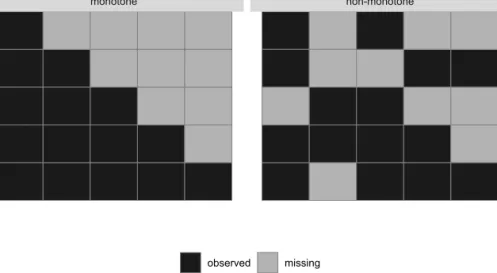
When values are missing in multiple variables, different patterns of missingness can arise. If variables can be ordered such that if a value is missing, the values of all variables following in the sequence are also always missing, the missing data pattern is calledmonotone (left panel of Figure 1.1). If such an order does not exist, the missing data pattern isnon-monotone(right panel of Figure 1.1). Monotone missing data patterns typically arise in longitudinal studies with drop-out, where once a patient has left the study, no further measurements are available. In studies where multiple variables measuring different aspects are obtained, either at the same time point or over time, non-monotone missing data patterns occur more frequently, since study participants do not return a particular questionnaire or miss a single visit to the research centre. In this thesis, we consider general, non-monotone missing data patterns.

1.2 Multiple Imputed Datasets

When the concept of multiple imputation was developed in the 1970s, a require-ment for a practical way to deal with missing data was that it allowed many researchers to analyse the incomplete data. Moreover, it was essential that these analyses could be done using only standard techniques and software tools, which required complete, balanced data, and without the need of in-depth knowledge of missing data methods (Scheuren 2005). Especially the second part of this re-quirement is still relevant today since analyses are often performed by researchers 6

(14)

1.2. Multiple Imputed Datasets

monotone non-monotone

observed missing

Figure 1.1: Visualization of a monotone and a non-monotone missing data pat-tern. Each column represents a variable, while rows represent different patterns of missing values.

without expert knowledge in statistics, who are usually only familiar with standard complete data methods and are not versed in Bayesian methodology.

Rubin’s solution to this practicality issue was to perform imputation once and to distribute the imputed data to various researchers. In this imputation procedure, multiply imputed, i.e., completed, versions of the original data were produced, which differed only in the values that had been filled in for the missing obser-vations. This allowed retaining some information on the uncertainty about the missing values, while each of the datasets could be analysed using standard meth-ods. Since the imputed datasets are not identical, the estimates obtained from the analysis of each dataset will vary. This variation in the obtained estimates allows assessing the additional uncertainty in the effect estimates that is caused by the missing values (Rubin 2004).

In the following, we first give an overview of some popular (Bayesian and non-Bayesian) methods that have been proposed for creating imputed values and then describe the most commonly used procedure to pool the results from the analyses of multiple imputed datasets.

(15)

1.2.1 Methods for Imputation

The task to create the imputed values requires to sample from the (posterior) predictive distribution of the unobserved data, given the observed data. Especially in larger datasets, with missing values in multiple variables, possibly of different measurement levels, and a non-monotone missing data pattern, this distribution is multivariate and not of any standard form.

Joint Model Imputation

Rubin’s suggestion in his initial paper on multiple imputation from 1977 (Rubin 2004) was to approximate the posterior predictive distribution with a multivariate normal distribution if variables are continuous, or with a multinomial distribution if data is categorical. Since sampling from either of these distributions is fast and readily available in software, this approach, especially using the multivariate normal distribution, is still used today (Carpenter and Kenward 2013). To allow for covariates of mixed type, the assumption is made that categorical variables have an underlying normal distribution and that different categories are observed depending on the value of that latent distribution. Due to its ability to impute incomplete baseline as well as time-varying covariates in multi-levels settings, we apply and investigate this approach in Chapter 5 of this thesis.

Expectation Maximization

A general approach that allows performing likelihood inference when parts of the data are unobserved, is theExpectation Maximization(EM) algorithm, introduced by Dempster et al. (1977). The algorithm alternates between the expectation (E) step, in which the expected value of missing data, conditional on observed data and current estimates of the parameters, is obtained, and the maximisation (M) step, in which parameter values are estimated by maximizing the likelihood of the parameters given the current values of the missing data. Even though the approach was not specifically developed to create multiple imputations, it could be applied in this way, if, once the algorithm has converged, not the expectation of missing values is determined, but instead multiple values are drawn from the estimated distribution. In settings where incomplete variables have non-linear associations with other variables, however, the distribution in the M-step may not have a closed form and updating the parameters becomes difficult.

Data Augmentation

Data augmentation, an approach similar to the EM algorithm, was proposed by Tanner and Wong (1987). It can be thought of as a Bayesian version of the EM 8

(16)

1.2. Multiple Imputed Datasets

algorithm since it has the same two-step structure, but the E step is replaced by imputation of missing values and the M step by estimation of the posterior distribution instead of maximization of the likelihood. The motivation behind augmenting the data is that sampling from p(θ | X) is often easier than sam-pling fromp(θ|Xobs)and works well if sampling ofp(Xmis |Xobs,θ)is possible. Nonetheless, even when Monte Carlo integration is used, sampling from distribu-tions that are not members of the exponential family may be difficult, diminishing the attractiveness of the approach. While Tanner and Wong (1987) aimed to es-timate the posterior distribution, Li (1988) focused on imputing values but used essentially the same algorithm.

The approach for analysis of incomplete data and imputation of missing values followed throughout this thesis uses data augmentation in conjunction with the Gibbs sampler. The joint distribution of all data, observed and unobserved, as well as the parameters, is specified in a sequence of univariate distributions. Us-ing Gibbs samplUs-ing, missUs-ing values are imputed by draws from the full conditional distributions arising from this joint distribution. Once the observed data is aug-mented by the imputed values, posterior inference for the parameters of interest can be obtained as if the data had been complete. The approach is described in detail in Chapter 2.

Multiple Imputation using Chained Equations

The nowadays most popular approach for creating multiple imputations, intro-duced by Van Buuren, Boshuizen, et al. (1999), also uses the idea of the Gibbs sampler but is a (mostly) frequentist approach. In multiple imputation using chained equations(MICE), also called multiple imputation using afully conditional specification (FCS), a full conditional distribution is specified for each incomplete variable and imputed values are sampled from these distributions. If a multivari-ate distribution exists that has the specified distributions as its full conditionals, the algorithm is a Gibbs sampler.

Specifying the full conditional distributions directly has the advantage that it allows for a flexible algorithm, in which distributions can be tailored to the mea-surement level of each variable, and sampling is performed on a variable by variable basis using samplers that are easy to implement. The MICE algorithm (Van Bu-uren 2012) starts by randomly drawing starting values from the set of observed values. Then, in each iteration t= 1, . . . , T, it cycles once through all incomplete variablesxj, j= 1, . . . , p. For each incomplete variablej, the currently completed data except xj is defined as X˙t₋j =

( ˙ xt 1, . . . ,x˙tj−1,x˙ t−1 j+1, . . . ,x˙tp−1 ) .The parame-ters of the model for xj, _θ˙t

j, are sampled from their distribution conditional on 9

(17)

the observed part ofxj and the currently completed data of the other variables from subjects that havexj observed:

p(θt_j|x_jobs,X˙₋j,R).

Imputed valuesx˙t_j are drawn from the predictive distribution of the missing values xmis_j given the other variables and parameters_θ˙t

j,

p(xmis_j |Xt₋_j,R,θt_j).

By filling in the imputed values of the last iteration, i.e., (x˙⊤1, . . . ,x˙⊤p )

into the original, incomplete, data, one imputed dataset is created. The algorithm is run multiple times with different starting values to create a set of multiply imputed datasets.

A drawback of the MICE algorithm is that there is no guarantee that a joint distri-bution exists that has the specified conditional distridistri-butions as its full conditionals. If no such distribution exists, the algorithm may not converge to the correct dis-tribution. Despite this theoretical limitation, it has been shown to work well in practice as long as the conditional distributions fit the data well enough (Zhu and Raghunathan 2015). In settings where incomplete covariates are involved in non-linear functional forms or interactions, or with complex outcomes, such as survival or longitudinal outcomes, specification of correct imputation models is often not feasible (Bartlett et al. 2015; Carpenter and Kenward 2013). Even specification of models that adequately include all information necessary to obtain valid impu-tations is not straightforward, and, in practice, often not even attempted when imputation is performed by researchers who are unaware that naive use of impu-tation software will lead to violation of important assumptions and thereby faulty imputations and biased inference. The performance of MICE when used naively for imputation of covariates in longitudinal data is the topic of Chapter 2 of this thesis.

1.2.2 Pooling Results from Multiple Imputed Datasets

Irrespective of the method used for producing imputations, the results from the analyses of the multiple imputed datasets need to be combined in a manner that takes into account the added uncertainty due to the missing values. The formulas for pooling of such results proposed by Rubin and Schenker (1986) (see also Rubin (1987)), usually referred to asRubin’s Rules, have gained wide acceptance and are outlined in the following.

For a parameter vector Q the overall estimate, pooled over the analyses of m

imputed datasets, can be calculated as the mean over the estimates from these 10

(18)

1.2. Multiple Imputed Datasets analyses, Q= 1 m m ∑ ℓ=1 b Qℓ,

where Qbℓ denotes the estimate obtained from theℓ-th imputed set. The overall variance of Qconsists of the within imputation variances W, which can be cal-culated by averaging over the estimated variances of the Qℓ from each imputed dataset,Wcℓ, W= 1 m m ∑ ℓ=1 c Wℓ,

and the between imputation variance, B, calculated as

B= 1 m−1 m ∑ ℓ=1 ( b Qℓ−Q ) ( b Qℓ−Q )⊤ .

Following Rubin and Schenker (1986), the total variance,T is the sum of within and between imputation variance, plus an additional termB/m, correcting for the finite number of imputations, i.e.,T=W+B+B/m. The relative increase in vari-ance that is due to the missing values can be estimated asrm= (B+B/m)/W. The (1 − α) 100% confidence interval for scalar Q can be calculated as

Q ± tν(α/2) √

T , where tν is the α/2 quantile of the t-distribution with

ν = (m−1)(1 +r−1 m

)2

degrees of freedom.

The corresponding p-value is the probability P r{F1,ν > (

Q0−Q )2

/T}, where

F1,ν is a random variable that has an F distribution with 1 and ν degrees of freedom, and Q0 is the null hypothesis value (typically zero).

In the above calculation, the degrees of freedomνare derived under the assumption that there are infinite degrees of freedom in the complete data, denoted νcom (Barnard and Rubin 1999). Since this is not a reasonable assumption for small datasets, Barnard and Rubin (1999) proposed a different calculation of the degrees of freedom for thet-distribution

˜ ν = ( 1 ν + 1 ˆ νobs )−1 =νm ( 1 + ν ˆ νobs )−1 =νcom [ {λ(νcom)(1−ˆγm)}− 1 +νcom ν ] where the observed-data degrees of freedom, νobs, are estimated as νˆobs =

λ(νcom)νcom(1− ˆγm), ˆγm = rm/(1 + rm) and λ(ν) = (ν + 1)(ν + 3). This small-sample version of Rubin’s Rules is implemented in theRpackage miceand used in this thesis.

(19)

1.3 The Bayesian Framework

Since the focus of this thesis is on inference for missing data under the Bayesian paradigm, in this section we will briefly introduce the Bayesian framework and some relevant concepts.

The idea behind the Bayesian paradigm is that inference about an unknown pa-rameter can be obtained by updating an initial guess or prior belief about that parameter with data (Bayes et al. 1763; Laplace 1774).

1.3.1 Bayes Theorem

Theposterior distribution, i.e., the distribution of a parameter θ conditional on the dataX, can be expressed as

p(θ|X) = ∫_∞p(X|θ)p(θ)

−∞p(X|θ)p(θ)dθ

.

In the above equations,p(θ)denotes theprior distributionofθ, i.e., the distribu-tion ofθthat is assumed without taking into account the collected data,p(X|θ) is thelikelihoodof the data given the parameter, and the denominator constitutes the marginal distribution of the data, i.e., the distribution of data under all possi-ble values ofθ, and is often called thenormalizing constant. Since this normalizing constant does not depend onθ, Bayes theorem is often simplified to

p(θ|X)∝p(X|θ)p(θ),

i.e., the posterior distribution is proportional to the product of the likelihood and the prior distribution.

In the Bayesian framework, the distribution relating unobserved values,Xmis, to observed values,Xobs, referred to by Rubin in his statement given above, is called theposterior predictive distribution of the missing data given the observed data,

p(Xmis |Xobs) = ∫

p(Xmis|Xobs,θ)p(θ|Xobs)dθ.

In practice, an analytic calculation of the posterior distribution is often not feasi-ble. In that case, it has to be approximated or determined numerically. A numeric method that is frequently used and works in complex settings is theMonte Carlo method.

(20)

1.3. The Bayesian Framework

1.3.2

Monte Carlo Methods

Instead of determining the posterior distribution analytically, the Monte Carlo method (Metropolis and Ulam 1949) draws random samples from it and uses these samples to calculate summary measures of the distribution, to approximate the corresponding measures of the posterior distribution.

Using the central limit theorem, the precision of this approximation to the sample mean,_θ¯_{, can be determined as}

¯

θ′±1.96sd(θ′)/√K,

where K is the number of independently sampled values θ′, and sd(θ′)/√K is called theMonte Carlo error.

In high-dimensional settings, however, even “just” sampling from the posterior distribution may not be feasible, since no sampler is available for direct sampling from a multivariate distribution of unknown form, and factorization of the distri-bution would require solving multiple integrals (Lesaffre and Lawson 2012). The development ofMarkov Chain Monte Carlomethods (Metropolis, Rosenbluth, et al. 1953; Hastings 1970) was crucial in overcoming this difficulty.

1.3.3 Markov Chain Monte Carlo

The idea behind Markov Chain Monte Carlo (MCMC) sampling is to construct a Markov chain that has the distribution to be sampled from as its stationary distribution. It is an iterative procedure in which a sequence of random variables is created by repeatedly drawing values from a distribution that depends on the previously drawn value. MCMC methods, hence, perform dependent sampling. By creating a Markov chain that has the posterior distribution as its stationary distribution, samples from that stationary distribution can, thus, be regarded as a sample from the posterior distribution.

1.3.4 Gibbs Sampler

The Gibbs sampler, introduced by Geman and Geman (1984), facilitates sam-pling from high-dimensional distributions by splitting a multivariate problem into a set of univariate problems. It uses the property that a joint distribution is fully specified by its corresponding set of full conditional distributions. Iteratively sam-pling from these, often univariate, distributions is usually relatively easy. Using Gibbs sampling to obtain draws in an MCMC chain, hence, allows sampling from high-dimensional posterior distributions.

(21)

1.3.5 Convergence, Mixing and Thinning

As previously mentioned, samples from an MCMC chain are only samples from the posterior distribution once the chain hasconverged, i.e., when the distribution of the values remains stable throughout further iterations. In order to obtain valid inferences, convergence of the chains must be checked, and, if necessary, samples from before the chain has converged need to be discarded. The iterations before the chain has converged are calledburn-inperiod.

Convergence may be checked visually, by plotting the drawn values against the it-eration number in a so-calledtraceplot, which should show a horizontal band with no apparent trends or patterns. In this thesis, we additionally evaluated conver-gence using a statistical criterion developed by Gelman and Rubin (1992). It uses multiple, independent chains for the same parameter, and compares within and between chain variances. When this criterion, which we refer to as the Gelman-Rubin criterionin the rest of this thesis, is close enough to one, say, no more than 1.2, the MCMC chains can be assumed to have converged.

Another potential issue when working with MCMC methods is that they perform dependent sampling. When this dependence is strong it can take many iterations before the MCMC chain converges and, moreover, many iterations until the chain has sufficiently explored the whole range of the posterior distribution. In order to provide enough information about the posterior distribution, a chain with high auto-correlation may have to be continued for more iterations than can practically be handled. To reduce the number of samples that have to be stored, a chain may be thinned out so that only a reduced number of samples is saved.

1.4 Motivating Datasets

The research presented in this thesis is motivated by several large cohort studies. Such studies are especially prone to missing values since typically a large number of variables are measured, and many variables are self-reported (i.e., by question-naire) or participants have to visit a research centre for measurements to be taken. Moreover, participants are from the general population and may not always see a direct personal benefit in complying with the study protocol.

Two datasets that were used in this thesis for demonstration of the statistical methods under investigation, as well as the real world application of the proposed approach, are briefly introduced in the following sections.

(22)

1.5. Outline of this Thesis

The Generation R Study

The Generation R Study (Kooijman et al. 2016) is an ongoing longitudinal population-based prospective cohort study from fetal life until young adult-hood, investigating growth development and health of children, conducted in Rotterdam, the Netherlands. Approximately 10000 pregnant women from the Rotterdam area with an expected delivery date between 2002 and 2006 were included and are followed up, together with their children, until the offspring is 18 years of age. Data is collected at scheduled visits to the research centre as well as by questionnaire, phone interviews or home visits, and augmented by registry information. Among other things, information on maternal diet and lifestyle, health and complications during pregnancy, child growth and health outcomes (e.g., asthma or infectious diseases), behaviour and cognition, body composition and obesity, and eye and tooth development, is collected at different time points. The National Health and Nutrition Examination Survey

The National Health and Nutrition Examination Survey (NHANES), conducted by the National Center for Health Statistics in the United States, is a large cohort of children and adults and investigates a broad range of health and nutrition related issues (National Center for Health Statistics (NCHS) 2011). Since 1999, a new cohort of approximately 5000 participants, chosen representatively of the US population, is included every year. Data on demographic, socioeconomic, dietary and health-related topics is obtained by interviews and physiological, dental and medical examinations, and laboratory tests are performed. The study is designed to, among other things, investigate risk factors for and prevalence of diseases, get insights into how nutrition (advice) may be used for disease prevention and to inform public health policies.

1.5

Outline of this Thesis

This section provides a brief overview of the content of the subsequent chapters. In Chapter 2 a fully Bayesian approach to analysis and imputation of data with incomplete covariate information is described in detail for the setting with a con-tinuous longitudinal outcome and incomplete baseline covariates.

Moreover, different approaches to the handling of a longitudinal outcome in mul-tiple imputation using MICE are investigated, both the naive but commonly used, and other, more sophisticated techniques. MICE and the fully Bayesian approach are compared using a simulation study and a real data example from the Gener-ation R Study, in which the associGener-ation between maternal diet during pregnancy 15

(23)

and gestational weight throughout pregnancy is analysed. This application is mo-tivated by the study conducted in Chapter 3.

Chapters 3 and 4 contain applications of the presented Bayesian approach us-ing data from the Generation R Study. In Chapter 3 the association between guideline-based (a priori) and data-driven (a posteriori) dietary patterns with gestational weight gain and trajectories of gestational weight are investigated. Us-ing the approach presented in Chapter 2, simultaneous analysis of the trajectories of gestational weight and imputation of incomplete baseline covariates is per-formed. The imputed data is then used in the secondary analysis to investigate the association of diet with weight gain.

Chapter 4 examines the effect of sugar containing beverage consumption by preg-nant women on body composition of their offspring. Measures of body composition are the body mass index (BMI), which was measured repeatedly, and the fat mass index and fat-free mass index, both measured when children where approximately six years of age. All three outcomes are modelled jointly, and imputation of in-complete baseline covariates is performed using the Bayesian approach presented in Chapter 2.

In Chapter 5, the approach of Chapter 2 is extended to time-varying covariates. Additional issues that arise with such covariates, specifically the potential endo-geneity and non-linear shape of the association with the outcome are considered. Advantages and disadvantages as well as the performance of the proposed ap-proach are compared to multiple imputation using a multivariate normal model in a simulation study and two research questions from the Generation R Study: the association between blood pressure and weight of mothers during pregnancy, and the association of maternal gestational weight and child BMI from birth until five years of age.

The implementation of our fully Bayesian approach to jointly analyse and impute incomplete data into the R package JointAIis described in Chapter 6. Func-tionality of the package to analyse incomplete data using generalized linear mixed models or generalized linear regression models, which may include non-linear forms or interaction terms, is demonstrated in detail. Data from the NHANES study as well as data simulated to mimic data from a longitudinal cohort study, such as the Generation R Study, is used to illustrate this functionality.

The thesis concludes in Chapter 7 with a general discussion of limitations of the proposed approach which arise from the model assumptions, and propositions as to how the approach and its implementation in software should be further improved and extended to facilitate valid inference with incomplete data in a wider range of applications and settings.

(24)

References

Andridge, R. R. and R. J. Little (2010). “A review of hot deck imputation for survey non-response”. International Statistical Review, 78(1):40–64. doi: 10. 1111/j.1751-5823.2010.00103.x.

Barnard, J. and D. B. Rubin (1999). “Miscellanea. Small-sample degrees of freedom with multiple imputation”.Biometrika, 86(4):948–955.doi: 10.1093/biomet/ 86.4.948.

Bartlett, J. W. et al. (2015). “Multiple imputation of covariates by fully conditional specification: accommodating the substantive model”. Statistical Methods in Medical Research, 24(4):462–487.doi: 10.1177/0962280214521348.

Bayes, T., R. Price, and J. Canton (1763). “An Essay towards solving a Problem in the Doctrine of Chances”.Philosophical Transactions,53:370–418.doi: 10. 1098/rstl.1763.0053.

Behrmann, H. I. (1954). “Sampling Technique in an Economic Survey of Sugar Cane Production”. South African Journal of Economics,22(3):326–336.issn: 1813-6982.doi: 10.1111/j.1813-6982.1954.tb01646.x.

Carpenter, J. R. and M. G. Kenward (2013). Multiple Imputation and its Appli-cation. John Wiley & Sons, Ltd. doi: 10.1002/9781119942283.

Dempster, A. P., N. M. Laird, and D. B. Rubin (1977). “Maximum likelihood from incomplete data via the EM algorithm”.Journal of the Royal Statistical Society. Series B (methodological), (1):1–38. url: http : / / www . jstor . org / stable/2984875.

Gelman, A. and D. B. Rubin (1992). “Inference from Iterative Simulation Us-ing Multiple Sequences”. Statistical Science, 7(4):457–472. doi: 10.1214/ss/ 1177011136.

Geman, S. and D. Geman (1984). “Stochastic Relaxation, Gibbs Distributions, and the Bayesian Restoration of Images”.IEEE Transactions on Pattern Analysis and Machine Intelligence, (6):721–741.doi: 10.1109/TPAMI.1984.4767596. Gorinson, M. (1969). “How the census data will be processed”. Monthly Labor

Review (pre-1986); Washington,92(12):42.url: http://www.jstor.org/stable/ 41837533.

Hastings, W. K. (1970). “Monte Carlo Sampling Methods Using Markov Chains and Their Applications”.Biometrika,57(1):97–109.doi: doi:10.2307/2334940. Kooijman, M. N. et al. (2016). “The Generation R Study: design and cohort update 2017”. European Journal of Epidemiology, 31(12):1243–1264. doi: 10 . 1007 / s10654-016-0224-9.

Laplace, P.-S. (1774). “Mémoire sur la probabilité des causes par les évènemens”. Mémoires de Mathématque et Physique, Presentés à l’Académie Royale des

(25)

Sciences, par divers Savans & lûs dans ses Assemblées, Tome Sixiéme,66:621– 56.

Lesaffre, E. M. and A. B. Lawson (2012). Bayesian Biostatistics. John Wiley & Sons.doi: 10.1002/9781119942412.

Li, K.-H. (1988). “Imputation using Markov chains”.Journal of Statistical Com-putation and Simulation, 30(1):57–79.

Little, R. J. and D. B. Rubin (2002).Statistical Analysis with Missing Data. Hobo-ken, New Jersey: John Wiley & Sons, Inc.doi: 10.1002/9781119013563. Metropolis, N., A. W. Rosenbluth, et al. (1953). “Equation of State Calculations

by Fast Computing Machines”.The Journal of Chemical Physics,21(6):1087– 1092.doi: 10.1063/1.1699114.

Metropolis, N. and S. Ulam (1949). “The Monte Carlo Method”. Journal of the American Statistical Association,44(247):335–341.doi: 10.2307/2280232. National Center for Health Statistics (NCHS) (2011).National Health and

Nutri-tion ExaminaNutri-tion Survey Data.url: https://www.cdc.gov/nchs/nhanes/. Nordbotten, S. (1963). “Automatic editing of individual statistical observations”.

Statistical Standards and Studies (3). United Nations Statistical Commission and Economic Commission for Europe. Conference of European Statisticians. url: http://hdl.handle.net/11250/178265.

Rubin, D. B. (1976). “Inference and Missing Data”.Biometrika, 63(3):581–592. doi: 10.2307/2335739.

— (1978a). “Bayesian Inference for Causal Effects: The Role of Randomization”. The Annals of Statistics,6(1):34–58.doi: 10.1214/aos/1176344064.

— (1978b). “Multiple Imputations in Sample Surveys - A Phenomenological Bayesian Approach to Nonresponse”. Proceedings of the Survey Research Methods Section of the American Statistical Association. Vol. 1. American Statistical Association, p. 20–34.

— (1987).Multiple Imputation for Nonresponse in Surveys. Wiley Series in Prob-ability and Statistics. Wiley.doi: 10.1002/9780470316696.

— (2004). “The Design of a General and Flexible System for Handling Nonre-sponse in Sample Surveys”. The American Statistician, 58(4):298–302. doi: 10.1198/000313004X6355.

Rubin, D. B. and N. Schenker (1986). “Multiple Imputation for Interval Estimation From Simple Random Samples With Ignorable Nonresponse”. Journal of the American Statistical Association,81(394):366–374.doi: 10.2307/2289225. Scheuren, F. (2005). “Multiple Imputation: How It Began and Continues”. The

American Statistician, 59(4):315–319.doi: 10.1198/000313005X74016. Tanner, M. A. and W. H. Wong (1987). “The Calculation of Posterior

Distribu-tions by Data Augmentation”.Journal of the American Statistical Association, 82(398):528–540.doi: 10.2307/2289457.

(26)

References

Van Buuren, S. (2012). Flexible Imputation of Missing Data. Chapman & Hall/CRC Interdisciplinary Statistics. Taylor & Francis.

Van Buuren, S., H. C. Boshuizen, and D. L. Knook (1999). “Multiple imputation of missing blood pressure covariates in survival analysis”.Statistics in Medicine, 18(6):681–694. doi: 10 . 1002 / (SICI ) 1097 0258(19990330 ) 18 : 6<681 :: AID -SIM71>3.0.CO;2-R.

Zhu, J. and T. E. Raghunathan (2015). “Convergence Properties of a Sequential Regression Multiple Imputation Algorithm”.Journal of the American Statisti-cal Association,110(511):1112–1124.doi: 10.1080/01621459.2014.948117.

(27)

(28)

2

Dealing with Missing Covariates in

Epidemiologic Studies

This chapter is based on

Nicole S. Erler, Dimitris Rizopoulos, Joost van Rosmalen, Vincent W. V. Jaddoe, Oscar H. Franco and Emmanuel M. E. H. Lesaffre. Dealing with missing covariates in epidemiologic studies: a comparison between multiple imputation and a full Bayesian approach. Statistics in Medicine, 2016;35(17), 2955 – 2974. doi:10.1002/sim.6944

(29)

2. Dealing with Missing Covariates in Epidemiologic Studies

Abstract

Incomplete data are generally a challenge to the analysis of most large studies. The current gold standard to account for missing data is multiple imputation (MI), and more specifically multiple imputation with chained equations (MICE). Numerous studies have been conducted to illustrate the performance of MICE for missing covariate data. The results show that the method works well in various situations. However, less is known about its performance in more complex models, specifically when the outcome is multivariate as in longitudinal studies. In current practice, the multivariate nature of the longitudinal outcome is often neglected in the imputation procedure or only the baseline outcome is used to impute missing covariates. In this chapter, we evaluate the performance of MICE using differ-ent strategies to include a longitudinal outcome into the imputation models and compare it with a fully Bayesian approach that jointly imputes missing values and estimates the parameters of the longitudinal model. Results from simulation and a real data example show that MICE requires the analyst to correctly specify which components of the longitudinal process need to be included in the imputa-tion models in order to obtain unbiased results. The fully Bayesian approach, on the other hand, does not require the analyst to explicitly specify how the longi-tudinal outcome enters the imputation models. It performed well under different scenarios.

(30)

2.1. Introduction

2.1

Introduction

Missing values are a common complication in the analysis of cohort studies. Since epidemiologic studies are often adjusted for a large number of possible confounders, the treatment of missing covariate values is of special interest and our focus in this chapter. There have been numerous publications that show that naive ways to handle missing data, like complete case analysis, often lead to biased estimates and considerable loss of power (Molenberghs and Kenward 2007; Donders et al. 2006; Janssen et al. 2010; Knol et al. 2010; Sterne et al. 2009; Van Buuren 2012). One standard approach to tackle this problem is to perform multiple imputation (MI) (Rubin 1987). Among the different flavours of MI, the Multiple Imputation with Chained Equations (MICE) (Van Buuren 2012) approach has gained the widest acceptance due to its good performance and ease of use. MI, and hence also MICE, works in three steps: First, a small number (often 5 or 10) of datasets are created by imputing each missing value multiple times. Each of the completed datasets can then be analysed using standard complete data methods. To obtain the overall result and to take additional uncertainty created by the missing values into account, the derived estimates are being pooled in the last step.

As a consequence of the separation of imputation and analysis steps, the relations between the outcome and the covariates, which are modelled in the analysis step, must be included explicitly in these imputation models. This means that the imputation models should not only contain other covariates in the predictor but also the outcome (Moons et al. 2006). When the outcome is univariate (and the model does not contain non-linear effects or interactions that involve incomplete covariates) this can be easily done because the outcome is just one of the variables in the dataset. However, when the outcome has a multivariate nature, such as the longitudinal outcome in our motivating study, it is not directly evident how this can be achieved, since longitudinal outcomes are often unbalanced with different subjects providing a different number of measurements at different time points. To overcome this problem one could consider simple or complex summaries of the long trajectories, such as including only a single value (e.g., baseline or the last available one) or the area under the trajectory. However, it is not clear which of these representations is the most adequate one for a specific analysis model and moreover, except in very simple situations, these summaries discard relevant information. As will be shown later, inclusion of inadequate summary measures of the subjects’ trajectories can lead to bias.

To prevent the problem of having to specify the appropriate summary measure in the MICE approach we propose here a fully Bayesian approach which com-bines the analysis model with the imputation models. The essential difference to 23

(31)

MICE is that by combining the imputation and analysis in one estimation pro-cedure, the Bayesian approach obtains inferences on the posterior distribution of the parameters and missing covariates directly and jointly. Thereby, the whole trajectory of the longitudinal outcome is implicitly taken into account in the im-putation of missing covariate values and no summary representation is necessary. A common approach to specify the joint distribution is to assume (latent) normal distributions for all variables and model it as multivariate normal (Carpenter and Kenward 2013; Goldstein et al. 2009). In the present work, we chose a different approach and follow Ibrahim et al. (2002), who propose a decomposition of the likelihood into a series of univariate conditional distributions. This produces the sequential fully Bayesian (SFB) approach which is a flexible and easy to implement alternative to MICE. Furthermore, since missing values are continuously imputed in each iteration of the estimation procedure, the uncertainty about the missing values is automatically taken into account and no pooling is necessary.

Besides approaches using multiple imputation or the fully Bayesian framework, other methods that can handle missing covariates in longitudinal settings have been investigated in the literature. Stubbendick and Ibrahim (2003), for instance, approach the missing data problem using a likelihood-based approach that factor-ized the joint likelihood into a sequence of conditional distributions, analogue the SFB approach. Other authors (Chen, Grace, et al. 2010; Chen and Zhou 2011) have shown how to apply weighted estimating equations for inference in settings with incomplete data.

In the present study, we describe different strategies to include a longitudinal outcome in MICE and compare them with the SFB approach. Both methods were evaluated using simulation and a motivating real data example that required the analysis of a large dataset with missing values in several variables of different types. The rest of this chapter is organized as follows: Section 2.2 briefly describes the data motivating this study. In Section 2.3 we introduce the problem of missing data, and describe and compare the two methods of interest, MICE and the SFB approach. Both methods are applied to a real data example in Section 2.4 and evaluated in a simulation study, which is described in Section 2.5. Section 2.6 concludes the chapter with a discussion.

2.2 Generation R Data

We have taken a subset of variables measured within the Generation R Study, a population-based prospective cohort study from early fetal life onwards in Rot-terdam, the Netherlands (Jaddoe et al. 2012), to illustrate both approaches. It was extracted with the aim to analyse the effect of diet, represented by three 24

(32)

2.2. Generation R Data

principal components, on gestational weight gain and contains a number of in-complete covariates of mixed type. The relationship between diet and weight gain during pregnancy is of special interest to epidemiologists because diet may influ-ence the amount of weight gained during pregnancy and subsequently affect the risk of adverse pregnancy outcomes. Furthermore, the Body Mass Index (BMI) before pregnancy is an important related factor on which general guidelines and recommendations for gestational weight gain are based.

variable 1 2 3 4 5 6 7 8 9 10 11 12 13 1: gender 2: dpa 3: dpb 4: dpc 5: age 6: height 7: parity 8: educ 9: smoke 10: alc 11: income 12: gsi 13: bmi

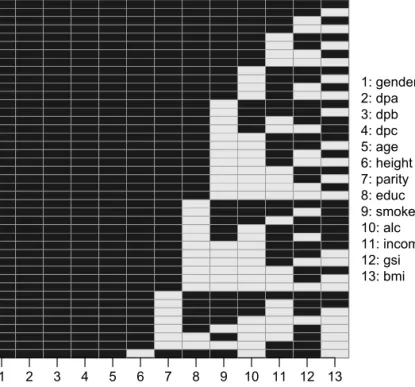
Figure 2.1: Missing data pattern of the Generation R data.

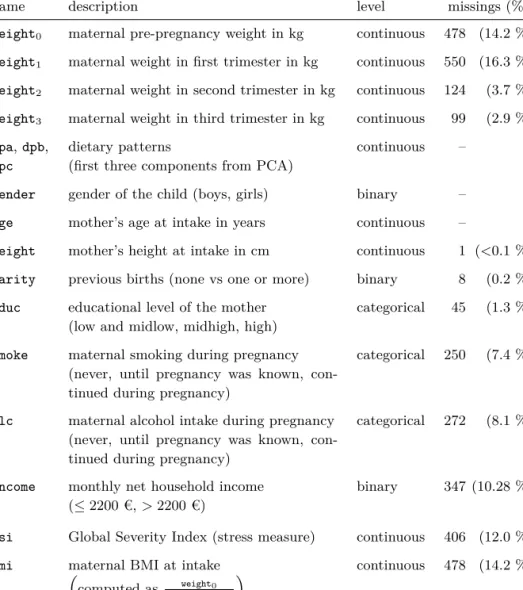
In the present study, data of 3374 pregnant women for whom dietary information was available, were analysed. Each woman was asked for her pre-pregnancy weight (baseline) and had up to three weight measurements during pregnancy, one in each trimester. There were 2297 women for whom all four weight measurements were recorded, 917 for whom three weight measurements were observed, 146 women had two measurements, and 14 women had only one measurement of weight. The gestational age at each measurement was recorded and the time point of the base-line measurement was set to be zero for all women. Table 2.1 in Appendix 2.A gives an overview of the available data. All covariates are cross-sectional. The variable bmiwas calculated from baseline weight (weight0) andheight. Except

(33)

forgender,ageand the dietary pattern variables, all variables had missing values, in proportions ranging between 0.03% and 14.17%. Reasons for missing covariate values in this study are usually (item) non-response in the questionnaires used. Missing baseline weight or weight measurement in the first trimester occurs when women are included in the study at a later gestational age. The missing pattern of the covariates is visualized in Figure 2.1. Variables 2 – 6, 12 and 13 are con-tinuous, variables 1, 7 and 11 are binary and variables 8 – 10 are categorical with three categories each. 2236 individuals had complete covariate data.

2.3 Dealing with Missing Data

A standard modelling framework for studying the relationship between a longitu-dinal outcomeyand predictor variablesXis a linear mixed model:

yij=x⊤ijβ+z⊤ijbi+εij,

whereyij is thej-th observation of individual i, measured at timetij,β denotes the vector of regression coefficients of the design matrix of the fixed effects Xi, where xij is a column vector that contains the j-th row of that matrix, and, analogously, zij denotes a row of the design matrix Zi of the random effectsbi and contains a subset of the variables inxij. Furthermore, the vectorbi follows a multivariate normal distribution with mean zero and covariance matrixD, and

εij is an error term that is normally distributed with mean zero and varianceσy2. In a complete data setting, the probability density function of interest isp(yij | xij,zij,θY|X), whereθY|X denotes the vector of parameters of the model. When some of the covariates are incomplete, X consists of two parts, the completely observed variablesXobsand those variables that containing missing values,Xmis. The measurement modelp(yij |xij,obs,xij,mis,zij,θY|X)then depends on unob-served data and standard complete data methods cannot be used any more. In this chapter, we restrict our attention to the imputation of cross-sectional co-variates. The missing data mechanism of the outcome is assumed to be ignorable, i.e., Missing At Random (MAR) or Missing Completely at Random (MCAR) (Lit-tle and Rubin 2002; Seaman, Galati, et al. 2013), and hence the missing outcome values do not require special treatment when using mixed effects models.

2.3.1 Multiple Imputation using Chained Equations

The underlying principle of MI is to divide the analysis of incomplete data into three steps: imputation, analysis and pooling. MICE is a popular implementation of the imputation step since it allows for multivariate missing data and does not 26

(34)

2.3. Dealing with Missing Data

require a specific missingness pattern. The idea behind MICE is that, under certain regularity conditions, the multivariate distribution

p(xi,mis|yi,xi,obs,θX), (2.1)

with xi,mis = (xi,mis1, . . . , xi,misp)⊤ and xi,obs = (xi,obs1, . . . , xi,obsq)⊤, can be

uniquely determined by its full conditional distributions and hence Gibbs sampling of the conditional distributions can be used to produce a sample from (2.1) (Van Buuren 2012). However, the MICE procedure does not actually start from a specification of (2.1), but it directly defines a series of conditional, predictive models of the form

p(xi,misℓ |xi,mis−ℓ,xi,obs,yi,θXℓ), (2.2)

that link each incomplete predictor variable xi,misℓ, ℓ = 1, . . . , p, with other

in-complete and in-complete predictors, xi,mis₋ℓ and xi,obs, respectively, and

impor-tantly with the outcome. These predictive distributions are typically members of the extended exponential family (extended with models for ordinal data) with linear predictor

gℓ {

E(xi,misℓ |xi,obs, xi,mis−ℓ,yi,γℓ,ξℓ,αℓ )}

=γ⊤_ℓxi,obs+ξ⊤ℓxi,mis₋ℓ+α⊤ℓf(yi),

wheregℓ(·)is the one-to-one monotonic link function for theℓ-th covariate andγℓ,

ξ_ℓ andαℓare vectors of parameters relating the complete and missing covariates and the outcome toxi,misℓ.

The functionf(·)specifies how the outcome enters the linear predictor. In the uni-variate case, the default choice forf(yi)is simply the identity function. However, when we have a multivariateyi, such as a longitudinal outcome, we cannot always simply specify α⊤_ℓyi because yi may have different length thanyk fori̸=k, and the time points tij andtkj of the observationsyij andykj may be very different. Hence, it is not meaningful to use the same regression coefficient αℓj to connect outcomes of different individuals with xi,misℓ and a representation needs to be

found that summarizes yi and that has the same number of elements which also have the same interpretation for all individuals.

(35)

2. Dealing with Missing Covariates in Epidemiologic Studies Some examples forf(yi)could be

f(yi) = 0, (2.3) f(yi) = yij, (2.4) f(yi) = 1 ni ni ∑ j=1 yij, (2.5) f(yi) = n∑i−1 j=1 (tij+1−tij) yij+yij+1 2 , (2.6) f(yi) = ˆbi=DbZe⊤i ( e ZiDbZe⊤i +Σbi )−1( yi−Xeiβˆ ) , (2.7) f(yi) = ∫ e Xi(t)βˆ+Zei(t)ˆbidt. (2.8)

Here, f(yi) from (2.3) results in omitting the outcome completely from the im-putation procedure. Equations (2.4) – (2.6) are examples of representations that directly use the observed outcome, where (2.4) uses only one observation, e.g., the first/baseline outcome ifj = 1, (2.5) uses the mean of the observed outcome and (2.6) uses the area under the observed trajectory to summarize yi. Func-tions (2.7) and (2.8) are examples of representaFunc-tions that are based on the fit of a preliminary model. Such a preliminary model could, for instance, include the time variable and possibly completely observed covariates. In (2.7) we use as a summary of the trajectory the empirical Bayes estimates of the random effects,_bˆ_i, whereXe andZe are the design matrices of the preliminary model and subsets ofX andZ, respectively,Σbi is the estimated covariance matrix of the error terms and

ˆ

β are the restricted maximum likelihood estimates of the regression coefficients from that model. Equation (2.8) describes the area under the estimated individual trajectory from (2.7).

Naturally, this list of possible summary functions is not exhaustive. In addition, combinations of these could be considered as well. Only in very simple settings is it possible to determine which function ofyiis appropriate. Carpenter and Kenward (2013) show that under a random intercept model foryi, (2.5) is the appropriate summary function in the imputation model for a normal cross-sectional covariate. For more complex analysis models or discrete covariates it is not straightforward to derive the appropriate summary functions.

In settings where the outcome is balanced or close to balanced and does not have a large number of repeated measurements, another approach could be to impute missing outcome values so that all individuals have the same number of 28

(36)

2.3. Dealing with Missing Data

measurements at approximately the same time points, and to include all outcome variables as separate variables in the linear predictor of the imputation models. Two important requirements that are necessary to obtain valid imputations using the MICE procedure as described above are that the imputation models need to be specified correctly and that the missing data mechanism needs to be ignorable, i.e., Missing Completely at Random (MCAR) or Missing At Random (MAR) (Little and Rubin 2002; Seaman, Galati, et al. 2013). In this case, the missing data mechanism does not need to be modelled specifically. A common assumption is that the missing values are MAR given all the observed values. This implies that also the values of the time variable of a mixed model should be included in the imputation models. Since the time variable is not constant over time, a summary representation has to be specified for this variable as well.

2.3.2

Fully Bayesian Imputation

The choice of a summary representation of a multivariate outcome can be avoided by using a fully Bayesian approach. In the Bayesian setting, the complete data likelihood is combined with prior information to compute the complete data pos-terior, which can be written as

p(θY|X,θX,xi,mis |yij,xi,obs) ∝ p(yij|xi,obs,xi,mis,θY|X)

p(xi,mis|xi,obs,θX)π(θY|X)π(θX), where θX is a vector containing parameters that are associated with the likeli-hood of the partially observed covariates Xmis andπ(θY_|X)andπ(θX)are prior distributions.

A convenient way to specify the joint likelihood of the missing covariates

p(xi,mis|xi,obs,θX) is to use a sequence of conditional univariate distributions (Ibrahim et al. 2002)

p(xi,mis1, . . . , xi,misp|xi,obs,θX) =

p(xi,mis1|xi,obs,θX1) p ∏ ℓ=2

p(xi,misℓ |xi,obs, xi,mis1, . . . , xi,misℓ−1,θXℓ), (2.9)

with θX = (θX1, . . . ,θXp)⊤. Each of these distributions is again chosen from

the extended exponential family, according to the type of the respective variable. Writing the joint distribution of the covariates in such a sequence provides a straightforward way to specify the joint distribution even when the covariates are of mixed type.

(37)

After specifying the prior distributionsπ(θY|X)andπ(θX), Markov chain Monte Carlo (MCMC) methods, such as Gibbs sampling, can be used to draw samples from the joint posterior distribution of all parameters and missing values. Since all missing values are imputed in each iteration of the Gibbs sampler, the additional uncertainty created by the missing values is automatically taken into account and no pooling is necessary.

The advantage of working with the full likelihood instead of the series of predic-tive models (2.2) is that we can choose how to factorize this full likelihood. More specifically, by factorizing the joint distribution p(yij,xi,mis,xi,obs | θY|X,θX) into the conditional distributionp(yij|xi,obs,xi,mis,θY|X)and the marginal dis-tribution p(xi,mis | xi,obs,θX), the joint posterior distribution can be specified without having to include the outcome into any predictor and no summary repre-sentationf(yi)is needed. This becomes clear when writing out the full conditional distribution of the incomplete covariates, used by the Gibbs sampler:

p(xi,misℓ |yi,xi,obs,xi,mis−ℓ,bi,θ)∝

p(xi,misℓ |xi,obs,xi,mis<ℓ,θXℓ)

{ _p

∏ k=ℓ+1

p(xi,misk |xi,obs,xi,mis<k,θXk)

} π(bi)π(θY_|X)π(θXℓ) p ∏ k=ℓ+1 π(θXk),

whereniis the number of repeated measurements of individuali,θ⊤Y|X = (γ⊤y,ξ⊤y),

θ⊤_X ℓ = (γ

⊤

ℓ,ξ⊤ℓ )and θ⊤Xk = (γ ⊤

k,ξ⊤k), andxi,mis<ℓ= (xi,mis1, . . . , xi,misℓ−1)⊤ and xi,mis<k= (xi,mis1, . . . , xi,misk−1)⊤denote the subset of variables in the sequence beforexi,misℓ andxi,misk, respectively.

The densities p(yij|xi,obs,xi,mis,bi,θY|X), p(xi,misℓ |xi,obs,xi,mis<ℓ,θXℓ) and

p(xi,misk|xi,obs,xi,mis<k,θXk) are members of the extended exponential family

with linear predictors 30

(38)

2.3. Dealing with Missing Data E(yij|xi,obs,xi,mis,bi,θY|X ) = γ⊤_yxi,obs+ξy⊤xi,mis+z⊤ijbi, (2.10) gℓ {

E(xi,misℓ |xi,obs,xi,mis<ℓ,θXℓ

)} = γ⊤_ℓxi,obs+ ℓ₋1 ∑ s=1 ξℓsxi,miss, (2.11) gk {

E(xi,misk|xi,obs,xi,mis<k,θXk

)} = γ⊤_kxi,obs+ k−1 ∑ s=1 ξksxi,miss, (2.12) k=ℓ+ 1, . . . , p.

Equation (2.10) represents the predictor of the linear mixed model, Equation (2.11) the predictor of the imputation model ofxmisℓ with link functiongℓ from the

ex-tended exponential family, and Equation (2.12) represents the predictors of the covariates that have xmisℓ as a predictive variable, with gk(·) being the

corre-sponding link function. As can easily be seen, none of the Equations (2.10) – (2.12) contains the outcome on its right-hand side, whereby the SFB approach avoids the need for a summary representation.

It has been mentioned before that it is not obvious how the imputation models in the sequence should be ordered (Bartlett et al. 2015) and, from a theoretical point of view, different orderings may result in different joint distributions, leading to different results. Chen and Ibrahim (2001) suggest to condition the categorical imputation models on the continuous covariates. In the context of MI it has been suggested to impute variables in a sequence so that the missing pattern is close to monotone (Van Buuren 2012; Schafer 1997; Bartlett et al. 2015). Our convention is to order the imputation models in (2.9) according to the number of missing values, starting with the variable with the least missing values. It has been shown, however, that sequential specifications, as used in the Bayesian approach, are quite robust against changes in the ordering (Chen and Ibrahim 2001; Zhu and Raghunathan 2015) and results may be unbiased even when the order of the sequence is misspecified as long as the imputation models fit the data well enough. Preliminary results of our own work (not shown here) indicated that our convention may lead to shorter computational times.

Like MICE, the SFB approach, in the form described above, is valid only under ignorable missing data mechanisms and when the analysis model, as well as the conditional distributions of the covariates, are correctly specified.

(39)

2.4 Data Analysis

2.4.1 Design

The data described in Section 2.2 was imputed and analysed using MICE and a frequentist linear mixed model as well as with the SFB approach.

The analysis model of interest was the linear mixed model

weight_ij =β0+β1genderi+β2dpai+β3dpbi+β4dpci+β5agei+

β6parity_i+β7educ2i+β8educ3i+β9smoke2i+

β10smoke3i+β11alc2i+β12alc3i+β13incomei+

β14gsii+β15bmii+β16timeij+β17timeij×dpai+

β18timeij×dpbi+β19timeij×dpci+β20time 2 ij+

bi0+bi1timeij+εij,

wheretimeis a centred version of the gestational age (in weeks) andbi0andbi1are correlated random effects. Interaction terms between the dietary pattern variables and time were included in the model to allow the slope of the weight trajectories to be associated with diet. The variable names used here are explained in Table 2.1 in Appendix 2.A.

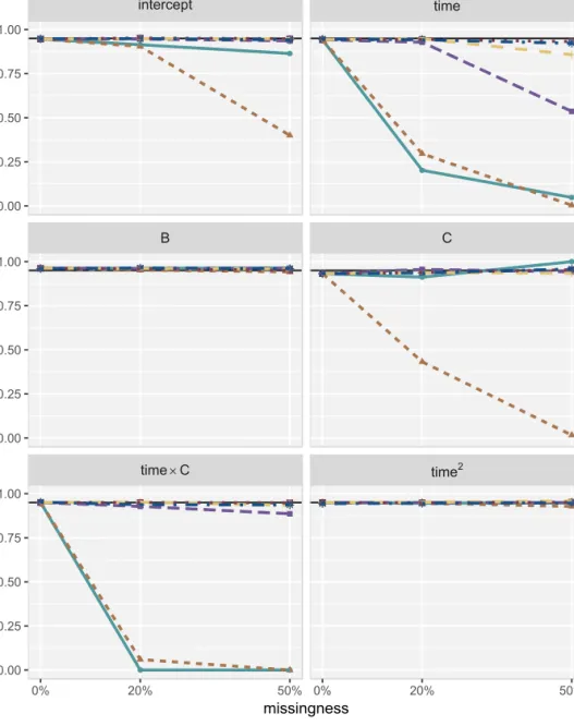
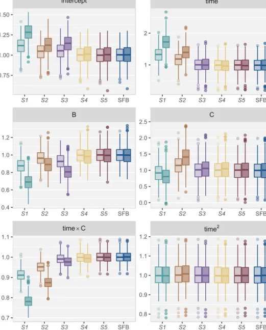
For the imputation with MICE, we chose five different strategies to representyi, three simple and commonly used strategies and two more sophisticated strategies: • S1: exclude the outcome from the imputation models, i.e.,f(yi)as in (2.3), • S2: include only the baseline outcome,weight0, i.e., f(yi)as in (2.4) with

j= 1,

• S3: include the mean of the observed weight measurements, i.e.,f(yi)as in (2.5),

• S4: obtain empirical Bayes estimates of the random effectsˆ_b_i _{from a} prelim-inary analysis model withtimeas only explanatory variable and a simplified random effects structure that only contained a random intercept, and include those estimates in the imputation, i.e.,f(yi)from (2.7) withbˆi= (ˆbi,0), • S5: fit a preliminary model with time as only explanatory variable, using

the random effects structure used in the analysis model, and include the empirical Bayes estimates from that model in the imputation step, i.e. f(yi) from (2.7) withˆ_b_i _{= (ˆ}_b_i,0_,ˆ_b

i,1).

For each of the five strategies, we calculatedf(weight_i)andf(timei), using the same functionf(·), and appended both as two or more new variables to the dataset. 32

(40)

2.4. Data Analysis

Since in our data the baseline value of time is zero for all individuals it does not help the imputation inS2and was hence not included in that strategy. Note that strategy S3 is implemented in the current version (2.22) of theR-package mice (Van Buuren and Groothuis-Oudshoorn 2011) for the imputation of continuous cross-sectional covariates in a 2-level model but not for variables of other type. It is also important to note that strategiesS1andS2may generally not lead to valid imputations since they do not include the entire outcome. They are included here to demonstrate the bias that may be introduced by a naive use of MICE.

Ten datasets were created for each strategy by taking the imputed values of the 20th iteration from the MICE algorithm using the R-package mice. Covariates were imputed according to their measurement level using (Bayesian) normal re-gression, logistic regression and a proport