high-dimensional data
Author
Kosuke Yoshida, Junichiro Yoshimoto, Kenji
Doya
journal or
publication title
BMC Bioinformatics
volume
18
page range
108
year
2017-02-14
Publisher
BMC
Rights
(C) 2017 The Author(s)
Author's flag
publisher
URL
http://id.nii.ac.jp/1394/00000206/
doi: info:doi/10.1186/s12859-017-1543-x
Creative Commons Attribution 4.0 International (http://creativecommons.org/licenses/by/4.0/)
M E T H O D O L O G Y A R T I C L E
Open Access
Sparse kernel canonical correlation
analysis for discovery of nonlinear interactions
in high-dimensional data
Kosuke Yoshida
1,2*, Junichiro Yoshimoto
3and Kenji Doya
2Abstract
Background: Advance in high-throughput technologies in genomics, transcriptomics, and metabolomics has created demand for bioinformatics tools to integrate high-dimensional data from different sources. Canonical correlation analysis (CCA) is a statistical tool for finding linear associations between different types of information. Previous extensions of CCA used to capture nonlinear associations, such as kernel CCA, did not allow feature selection or capturing of multiple canonical components. Here we propose a novel method, two-stage kernel CCA (TSKCCA) to select appropriate kernels in the framework of multiple kernel learning.
Results: TSKCCA first selects relevant kernels based on the HSIC criterion in the multiple kernel learning framework. Weights are then derived by non-negative matrix decomposition with L1 regularization. Using artificial datasets and nutrigenomic datasets, we show that TSKCCA can extract multiple, nonlinear associations among high-dimensional data and multiplicative interactions among variables.
Conclusions: TSKCCA can identify nonlinear associations among high-dimensional data more reliably than previous nonlinear CCA methods.
Keywords: Kernel canonical correlation analysis, Hilbert-Schmidt independent criterion, L1 regularization
Background
Canonical correlation analysis (CCA) [1] is a statistical method for finding common information from two differ-ent sources of multivariate data. This method optimizes linear projection vectors so that two random multivari-ate datasets are maximally correlmultivari-ated. With advances in high-throughput biological measurements, such as DNA sequencing, RNA microarrays, and mass spectroscopy, CCA has been extensively used for discovery of inter-actions between the genome, gene transcription, protein synthesis, and metabolites [2–5]. Because CCA solution is reduced to an eigenvalue problem, multiple compo-nents of interactions with sparse constraints are readily introduced [4, 6, 7].
Kernel CCA (KCCA) was introduced to capture non-linear associations between two blocks of multivariate *Correspondence: [email protected]
1Graduate School of Informatics, Kyoto University, Kyoto, Japan 2Neural Computation Unit, Okinawa Institute of Science and Technology, Okinawa, Japan
Full list of author information is available at the end of the article
data [8–11]. Given two blocks of multivariate dataxandz, KCCA finds nonlinear transformationsf(x)andg(z)in a reproducing kernel Hilbert space (RKHS) so that the cor-relation betweenf(x)andg(z)is maximized. In order to avoid overfitting and to improve interpretability of results, sparse additive functional CCA (SAFCCA) [12] constrains f(x) and g(z) as sparse additive models and optimizes them using the biconvex back-fitting algorithm [13]. How-ever, it is not straightforward to obtain multiple orthog-onal transformations for extracting multiple components of associations. Another method for finding nonlinear associations is to maximize measures of nonlinear match-ing, such as the Hilbert-Schmidt Independent Criterion (HSIC) [14] and the Kernel Target Alignment (KTA) [15] between linearly projected datasets xandz[16]. While these methods can obtain multiple orthogonal projec-tions by iteratively analyzing residuals, it is impossible for these methods to remove irrelevant features, making them prone to overfitting.
In this paper, we propose two-stage kernel CCA (TSKCCA), which enables us (1) to select sparse features © The Author(s). 2017Open AccessThis article is distributed under the terms of the Creative Commons Attribution 4.0 International License (http://creativecommons.org/licenses/by/4.0/), which permits unrestricted use, distribution, and reproduction in any medium, provided you give appropriate credit to the original author(s) and the source, provide a link to the Creative Commons license, and indicate if changes were made. The Creative Commons Public Domain Dedication waiver (http://creativecommons.org/publicdomain/zero/1.0/) applies to the data made available in this article, unless otherwise stated.
in high-dimensional data and (2) to obtain multiple non-linear associations. In the first stage, we represent target kernels with a weighted sum of pre-specified sub-kernels and optimize their weight coefficients based on HSIC with sparse regularization. In the second stage, we apply stan-dard KCCA using target kernels obtained in the first stage to find multiple nonlinear correlations.
We briefly review CCA, KCCA, and two-stage MKL, and then present TSKCCA algorithm. We apply TSKCCA to three synthetic datasets and nutrigenomic experimen-tal data to show that the method discovers multiple nonlinear associations within high-dimensional data, and provides interpretation that are robust to irrelevant fea-tures.
CCA, kernel CCA, and multiple kernel learning
In this section, we briefly review the bases of our pro-posed method, namely, linear canonical correlation anal-ysis (CCA), kernel CCA (KCCA), and multiple kernel learning (MKL).
Canonical correlation analysis (CCA)
LetD= {(xn,zn)}Nn=1beNpairs of samples, wherexnand znare then-th samples drawn fromp- andq-dimensional Euclidian space, respectively. Letfw(x)≡wTxandgv(z)≡ vTzdenote the projection ofx∈ Rpbyw∈ Rpand that ofz∈ Rqbyv ∈Rq, respectively. The objective of linear CCA is to find projections that maximize Pearson’s corre-lation betweenFw ≡ {fw(xn)}Nn=1andGv ≡ {gv(zn)}Nn=1 and formulated as the following optimization problem:
max
w∈Rp,v∈Rq Cov(Fw,Gv) (1a)
subject to Var(Fw)=Var(Gv)=1, (1b) where Var(·) and Cov(·,·) denote the empirical variance and covariance of the data, respectively. The optimal solu-tion (w∗,v∗) of Eq. (1a and 1b) is obtained by solving generalized eigenvalue problems and successive eigen-vectors represent multiple components. The projections, f∗(x) = w∗Txandg∗(z) =v∗Tz, are said to be canonical variables forx∈Rpandz∈Rq, respectively. If we intro-duce sparse regularization on wandv, we obtain sparse projections [4, 6, 7].
Kernel CCA
In Kernel CCA (KCCA), we suppose that the original data are mapped into a feature space via nonlinear functions. Then linear CCA is applied in the feature space. More specifically, nonlinear functionsφx : Rp → Hx andφz :
Rq→H
ztransform the original data{(xn,zn)}Nn=1to fea-ture vectors {(φx(xn),φz(zn))}Nn=1 in reproducing kernel Hilbert spaces (RKHS)HxandHz. Inner-product kernels forHxandHzare defined askx(x,x)=φx(x)Tφx(x), and kz(z,z)=φz(z)Tφz(z).
Let us implementfw(x)andgv(z)by projectionsfw(x)≡ wTφx(x)andgv(z)≡vTφz(z). By introducing appropriate regularization terms, Eq. (1a and 1b) can be reformulated as the following optimization problem ([8, 9]):
max α∈RN,β∈RN α TK xKzβ (2a) subject to αT Kx+ Nκ 2 I 2 α=1 (2b) βT Kz+ Nκ 2 I 2 β=1, (2c)
whereKx andKzareN-by-N kernel matrices defined as [Kx]nn=kx(xn,xn)and [Kz]nn=kz(zn,zn)1.Iis theN -by-N identity matrix andκ(κ > 0) is the regularization parameter.
Once having obtained the solution of Eq. (2a–2c), denoted by(α∗,β∗), canonical variables forx ∈ Rpand z∈Rqare given by f∗(x)= N n=1 kx(x,xn)αn∗ (3a) g∗(z)= N n=1 kz(z,zn)βn∗, (3b)
respectively. As indicated by Eq. (2a–2c), the nonlinear functions,φxandφz, are not explicitly used in the compu-tation of KCCA. Instead, the kernelskxandkzimplicitly specify the nonlinear functions, and the main goal is to solve the constrained quadratic optimization problem with 2N-dimensional variables.
Multiple kernel learning
Kernel methods usually require users to design a particu-lar kernel, which critically affects the performance of the algorithm. To make the design more flexible, the frame-work of multiple kernel learning (MKL) was proposed for classification and regression problems [17, 18]. In MKL, we manually designMxsub-kernels{kx(m)}Mm=x1, where each sub-kernel kx(m) uses only a distinct set of features inx. Also, Mz sub-kernels {kz(l)}Ml=z1 for z is also designed in the same manner. Then,kxandkzare represented as the weighted sum of those sub-kernels:
kx(x,x)= Mx m=1 ηmkx(m)(x,x) (4a) kz(z,z)= Mz l=1 μlkz(l)(z,z), (4b) where weight coefficients of sub-kernels, {ηm}Mm=x1 and {μl}Ml=z1are tuned to optimize an objective function.
A specific example of this framework is the two-stage MKL approach [15, 19]: In the first stage, the weight coef-ficients are optimized based on a similarity criterion, such as the kernel target alignment; then, a standard kernel algorithm, such as support vector machine, is applied in the second stage.
Methods
In this section, we propose a novel nonlinear CCA method, two-stage kernel CCA (TSKCCA), inspired by the concepts of sparse multiple kernel learning and kernel CCA. In the following, we present the general framework of TSKCCA, followed by our solutions for practical issues in the implementation.
First stage: multiple kernel learning with HSIC and sparse regularizer
In TSKCCA, sub-kernels are restricted to the same class as Eq. (4a and 4b), allowing us to express the kernel matricesKxandKzas Kx= Mx m=1 ηmKx(m) (5a) Kz= Mz l=1 μlKz(l), (5b) where [Kx(m)]nn= kx(m)(xn,xn) and [Kz(l)]nn= k(zl)(zn,zn). The goal of the first stage is to opti-mize the weight vector η = (η1,. . .,ηMx)T and
μ = (μ1,. . .,μMz)T so that kernel matricesKx andKz
statistically depend on each other as much as possible, while irrelevant sub-kernels are filtered out.
The statistical dependence betweenKx andKzis eval-uated by the Hilbert-Schmidt Independent Criterion (HSIC) and approximated by its empirical estimator [14]:
D(Kx,Kz)=
Tr(KxHKzH)
(N−1)2 , (6)
whereHis anN-by-Nmatrix such that [H]nn=δnn−N1, andδnn is Kronecker’s delta. Tr(·)denotes the trace. In our setting, optimization problem is reduced to a simple biliear form with respect toηandμ:
D(Kx,Kz)=ηTMμ, (7)
whereMis aMx-by-Mzmatrix such that [M]ml=
Tr(Kx(m)HKz(l)H)
(N−1)2 . (8)
In addition to maximizing the dependency measure D(Kx,Kz),ηandμshould be sparse in order to filter out irrelevant sub-kernel matrices. To this end, we determine
optimal weight vectors as the solution of the following constrained optimization problem:
max η∈RMx,μ∈RMz D(Kx,Kz)=η TMμ (9a) subject to η≥0,μ≥0, η2= μ2=1, (9b) η1≤c1,μ1≤c2, (9c) wherexp=(i|xi|p)1/pis theLp-norm of the vectorx andc1andc2are parameters (See also “Parameter tuning by a permutation test” section). This optimization prob-lem is an example of penalized matrix decomposition with non-negativity constraints [4]. Accordingly, we can obtain optimal weight coefficients by performing singular value decomposition of matrixMunder constraints. In this pro-cess, thei-th left singular vectorη(i)=(η1(i),. . .,ηM(i)
x)
Tas well as the right singular vectorμ(i) = (μ(1i),. . .,μ(Mi)z)T are obtained iteratively by Algorithm 1.
Algorithm 1 Penalized Matrix Decomposition for Learning Kernels
Input:M(Eq. 8), regularizationc1andc2 fori=1torank(M)do
initializeηito a first left singular vector ofM repeat μ(i)← S((η(i)TM)+,) S((η(i)TM)+,) 2 η(i)← S((Mμ(i))+,) S((Mμ(i))+,)2 untilConvergence
computei-th singular value asσi←η(i)TMμ(i) obtain residual asM←M−σiη(i)μ(i)T end for Output:{μ(i)}rank(Mx) i=1 and{η(i)} rank(Mz) i=1
In Algorithm 1, S denotes the element-wise soft-thresholding operator: Them-th element ofS(a,c)is given by sign(am)(|am| −c)+, where(x)+isxifx≥ 0 and 0 if x<0. In each step,is chosen by a binary search so that L1 constraintsη1 ≤c1andμ1 ≤c2are satisfied. In general, the above iteration does not necessarily converge to a global optimum. For each iteration, we initializeη(i) with a non-sparse, left singular vector ofM, following the previous study, to obtain reasonable solutions [4].
The second stage: kernel CCA
After learning kernels via penalized matrix decomposition as above, we perform the second stage of standard ker-nel CCA [8, 9] to obtain optimal coefficientsα∗ andβ∗ (Eq. 3a and 3b) with parameterκ for each pair of singu-lar vectors{η(i),μ(i)}ranki=1(M). Given test kernel{Kx(,mtest) }Mx
and {Kz(,ltest) }Mz
l=1, test correlation corresponding to the i -th singular vectors is defined as correlation between
Mx m=1ηmKx(m,test) α∗and Mz l=1μlK (l) z,testβ∗.
Practical solutions for TSKCCA implementation
TSKCCA still has several options for sub-kernels to be designed manually. In this study, we focus on feature-wise kernel and pair-feature-wise kernel defined in the following sections.
Feature-wise kernel
Feature-wise kernel was introduced to perform feature-wise nonlinear Lasso [20]. In the previous study, using feature-wise kernels as sub-kernels in sparse MKL resulted in sparsity in terms of features since each sub-kernel corresponds to each feature. With xnm and znl representing them-th feature forxn andl-th feature for zn, respectively, we adopt the following Gaussian kernel in this study: [Kx(m)]nn =exp −γx(xnm−xnm)2 (10a) [Kz(l)]nn =exp −γz(znl−znl)2 , (10b)
where γx and γz are width parameters. By applying feature-wise kernels, projection functions are restricted to additive models defined as f∗(x) = mp=1fm(x.m) and g∗(z) = ql=1gl(z.l), wherefm : R → R(m = 1,. . .,p) and gl : R → R (l = 1,. . .,q) are certain nonlinear functions2. Note that the number of sub-kernels,M
xand Mz, are equivalent to the number of features, pand q, respectively.
Pair-wise kernel
We introduce pair-wise kernels as sub-kernels to consider cross-feature interactions among all possible pairs of fea-tures. Since the sparseness is induced to the weight of sub-kernels, the pair-wise kernels result in selecting rel-evant cross-feature interactions. Projection functions are defined as f∗(x) = pm<mfm,m(x.m,x.m) andg∗(z) = q
l<lgl,l(z.l,z.l), wherefm,m : R2 →Randgl,l : R2 → Rare certain nonlinear functions with two dimensional inputs. Note that the number of sub-kernels,MxandMz, are,p(p−1)/2 andq(q−1)/2, respectively.
Preprocessing for MKL
We normalize the sub-kernels to have uniform variance in RKHS. This is an important procedure in the context of MKL because each feature-wise kernel has a different scale. This makes it difficult to evaluate weight coefficients
[21]. To compensate for that, we calculate the varianceσ2 in RKHS as σ2= 1 N N n φ (xn)− 1 N N n φ (xn) 2 2 (11a) = 1 N N n φ (xn)Tφ (xn)− 1 N2 N n,n φ (xn)Tφ (xn) (11b) = 1 N N n [K]nn− 1 N2 N n,n [K]nn. (11c)
Dividing each sub-kernel by its varianceK → σK2, we can achieve normalization of each sub-kernel.
Parameter tuning by a permutation test
When the kernel matrixKx (orKy) is full rank, as is typ-ically our case, KCCA with a smallκ (κ 1) can always find a solution such that the maximum canonical corre-lation nearly equals one. This property makes it difficult to tune the regularization parameters for the first stagec1 andc2. To solve the issue, we introduce a simple heuristics. The key idea is to conduct a permutation test for decid-ing whether to reject a null hypothesis that the maximal canonical correlation induced byi-th singular vectors is no more than those attained whenxandzare statistically independent. Since thep-value of this test is interpreted as the deviance between the actual outcome and those expected under the null hypothesis, we use it as a score to evaluate the significance ofi-th singular vectors where smallerp-value is more significant.
Algorithm 2 summarizes our implementation for the permutation test. Only for the first singular vectorsη(1) and μ(1), this procedure is applied to various pairs of (c1,c2)that satisfy the constraints of 1≤ c1 ≤√Mxand 1≤c2≤ My[4]. Among them, the pair with the lowest p-value is chosen as the optimal parameters ofc1andc2.
Algorithm 2A Permutation Test Input:{Kx(m)}Mm=x1,{K (l) z }Ml=z1,c1, andc2 c=Cor({Kx(m)}Mm=x1,{K( l) z }Ml=z1,η(i),μ(i)) forb=1toBdo
permute the samples ofxand calculate{ ˜Kx(m)}Mm=x1 obtainM˜ where [M˜]ij= Tr(
˜
Kx(m)HKz(l)H)
(N−1)2
perform the first stage; matrix decomposition ofM˜ to obtainη˜(i)andμ˜(i) calculatecb=Cor({ ˜Kx(m)}Mm=x1,{K (l) z }Ml=z1,η˜(i),μ˜(i)) end for p= B b=1I(|cb|>|c|) B+1 Output:p
For simplicity, other parameters, such asγ in the Gaus-sian kernel andκin KCCA, are fixed heuristically.γ−1is set to the median of the Euclidean distance between data points andκis set to 0.02 as recommended in the previous study [9].
Results
In this section, we experimentally evaluate the perfor-mance of our proposed TSKCCA, SAFCCA [12], and other methods using synthetic data and nutrigenomic experimental data.
Dataset 1: single nonlinear association
To evaluate the ability to extract a single nonlinear associ-ation, we generated simple synthetic data which consisted of a single pair of relevant features in quadratic associ-ation and noise, in which standard CCA and KCCA are known to performance poorly [12]. LetN(μ,s2)andU(A) denote the normal distribution with mean μ, variance s2, and uniform distribution supported inA, respectively. The synthetic data were generated as
x.m ∼ U([−0.5, 0.5]) m=1,. . .,D z.1 = x2.1+
z.l ∼ U([−0.5, 0.5]) l=2,. . .,D
∼ N(0,s2),
whereDwas the total number of dimensions and was independent noise.
The optimal model in each method was trained usingN training samples. Here, we assumedc1 = c2in the range of 1 ≤ c1,c2 ≤
√
D
2 and obtained optimal values using a permutation test with B = 100. The test correlation
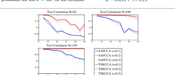
was evaluated with separate 100 test samples, averaged over 100 simulation runs as we varied the number of dimensions, the sample size, and the noise level.
Figure 1 shows the test correlations achieved by TSKCCA and SAFCCA with different data dimensionsD, sample size N, and noise level s. In the first stage, our method selected only two sub-kernels, corresponding to x1andz1, among 2×Dsub-kernels in the first stage, espe-cially in the case ofN =100 andN =150. As a result, it achieved better test correlation than SAFCCA, especially with high-dimensional data, indicating that our method was sufficiently robust.
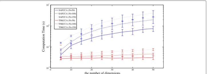
In addition, Fig. 2 shows average computation time for each method over 100 simulation runs with dataset 1. Computation time of TSKCCA was comparable with that of SAFCCA, and could scale up with the feature size. Note that all the experiments were performed on a Mac-Book Pro with Intel Core i7 (2.9 GHz dual core processor with 4 MB L3 cache) with 8 GB main memory. All the simulation programs were implemented in MATLAB®.
Dataset 2: multiple nonlinear associations
To test whether our method could extract multiple non-linear associations precisely, we generated the following data: x.m ∼ U([−0.5, 0.5]) m=1,. . ., 25 z.1 = x.1+exp(−x2.4)+1 z.2 = x2.2+sin(πx.5/2)+2 z.3 = |x.3| +1/(1+exp(−5x.6))+3 z.l ∼ U([−0.5, 0.5]) l=4,. . ., 25 l ∼ N(0, 0.12) l=1, 2, 3.
Fig. 1Comparison of test correlation averaged over simulation runs in Data 1. The horizontal axis denotes the number of dimensionsD, and the
vertical axis denotes test correlations. The number of training samples is 50, 100, and 150. TSKCCA outperforms SAFCCA, especially with high-dimensional data
Fig. 2Comparison of computation time for Data 1. The horizontal axis denotes the number of dimensionsD, and the vertical axis denotes computation time in log-scale. The number of training samples is 50, 100, 150 for SAFCCA and TSKCCA. Computation time of TSKCCA is moderate and can be scaled
First, we performed a permutation test withB = 1000 for ten singular vectors{η(i),μ(i)}10
i=1corresponding to the ten highest singular values ofMgiven by Eq. (8).P-values of the top three were significant (p< 0.001) and the rest were non-significant. This result suggests that only the three singular vectors included nonlinear associations.
Figure 3 shows the transformations f(x) and g(z) obtained with TSKCCA. In the first singular vectors, the contributions of η11, η41 andμ11 were dominant, indicat-ing thatx.1,x.4andz.1were associated. The contributions
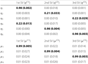
ofη22,η25andμ22in the second singular vectors were also dominant, indicating thatx.2,x.5andz.2were associated. Finally, the contributions ofη33,η36andμ33in the third sin-gular vectors were dominant, indicating thatx.3,x.6andz.3 were associated. Some singular vectors averaged over 100 simulation runs are listed in Table 1. Our results suggest that TSKCCA achieved feature selection precisely.
We further evaluated test correlation, precision, and recall averaged over 20 simulation runs. Table 2 shows that SAFCCA failed to detect all relevant features because it is
Fig. 3Transformationsf(x)andg(z)obtained with TSKCCA. The top three rows and the bottom row show the resulting functions corresponding to
Table 1Feature selection through singular vectors (SVs) in data 2 1st SV (η(1)) 2nd SV (η(2)) 3rd SV (η(3)) η1 0.98 (0.002) 0.00 (0.018) 0.00 (0.001) η2 0.00 (0.003) 0.21 (0.033) 0.00 (0.001) η3 0.00 (0.001) 0.00 (0.010) 0.22 (0.029) η4 0.22 (0.013) 0.00 (0.017) 0.00 (0.005) η5 0.00 (0.000) 0.98 (0.004) 0.00 (0.005) η6 0.00 (0.004) 0.00 (0.002) 0.98 (0.003) 1st SV (μ(1)) 2nd SV (μ(2)) 3rd SV (μ(3)) μ1 0.99 (0.005) 0.01 (0.022) 0.01 (0.014) μ2 0.01 (0.027) 0.99 (0.004) 0.01 (0.015) μ3 0.01 (0.024) 0.01 (0.018) 0.99 (0.003) μ4 0.01 (0.023) 0.01 (0.026) 0.01 (0.017)
These results show mean weight coefficients (standard deviation) in 100 simulation runs. Significant weight coefficients are bold faced
not able to obtain multiple canonical correlations, while our method detected 9 relevant sub-kernels out of 50 in the first stage in most runs. Note that the precision is the fraction of retrieved features that are relevant and recall is the fraction of relevant features that are retrieved.
Dataset 3: feature interactions
To assess the capability of TSKCCA in discovering non-linear interactions, we generated data with a product term:
x.m ∼ U([−0.5, 0.5]) m=1,. . .,D z.1 = x.1x.2+
z.l ∼ U([−0.5, 0.5]) l=2,. . .,D
∼ N(0, 0.12),
whereDwas the number of dimensions. For this dataset, we used feature-wise kernels and pair-wise kernels as sub-kernels in order to handle both single feature effects and cross-feature interactions like the termx.1x.2. There were D+D×(D−1)/2 sub-kernels, the weight coefficients of which were optimized in our method.
Table 2Comparison of test correlation, precision, and recall in
data 2
Correlation Precision Recall
TSKCCA 0.9670 0.9163 1
0.9636 0.9732
SAFCCA 0.7585 0.6350 0.4375
TSKCCA can identify most relevant features through three significant singular vectors, while SAFCCA can only identify a small set of them
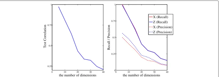
First, to evaluate the performance of our method with feature-wise and pair-wise kernels, we obtained test cor-relations evaluated by individual test data (N = 100) in different numbers of dimensionsD. Next, to evaluate the accuracy of feature selection of the model, we assessed recall and precision. Average test correlations, recall, and precision over 100 simulation runs are shown in Fig. 4. Our results illustrate that in the case ofD < 10 (i.e. the number of sub-kernels is less than 10+10×9/2 = 55), our method successfully determined the relation between z.1andx.1x.2.
Dataset 4: nutrigenomic data
We then analyzed a nutrigenomic dataset from a previ-ous mprevi-ouse study [22, 23]. In this study, expression of 120 genes in liver cells that would be relevant in the context of nutrition and concentrations of 21 hepatic fatty acids were measured on 20 wild-type mice and 20 PPARα-deficient mice. Mice of each genotype were fed 5 different diets with different levels of fat. For matrix notation, gene expression data were denoted byX ∈ R40×120, and data regarding concentrations of fatty acids was denoted byZ ∈R40×21. Data were standardized to have a mean of zero and unit variance in each dimension. Several linear correlations betweenXandZwere detected by applying a regularized version of the linear CCA [5, 23].
First, we performed a permutation test for sparse CCA, KCCA, SAFCCA, and TSKCCA on parameters defined by equally-spaced grid points in order to identify signif-icant associations in these data. In KCCA and SAFCCA, there were no significant associations; thus, we focused on sparse CCA and TSKCCA in the following analysis. We identified two significant linear associations in sparse CCA (p < 0.001 using a permutation test) and one nonlinear association in TSKCCA (p = 0.0067 using a permutation test) withc1=2.6257 andc2=1.9275.
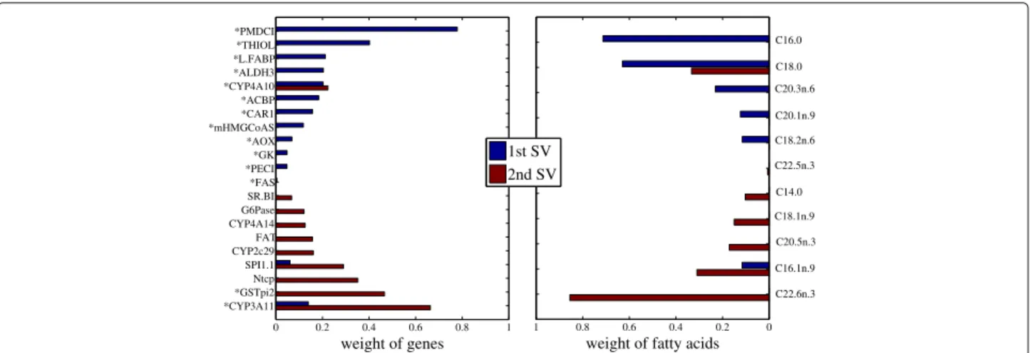
Figures 5 and 6 show the results of feature selection of sparse CCA and TSKCCA, respectively. Genes selected by the first singular vector of our method have dif-ferent expression levels in difdif-ferent genotypes (marked with asterisk), suggesting that our method successfully extracted the nonlinear correlation associated with geno-types.
For further analysis, cross-validation was performed in 100 runs. In each run, 40 samples were randomly split into 30 training samples used for fitting models and 10 validation samples used for evaluating the canonical cor-relation for fitted models. Figure 7 shows box plots of correlation coefficients in sparse CCA and TSKCCA. Left one represents the first canonical correlation coefficient in sparse CCA and right one represents correlation coef-ficient obtained with the first singular vectors. Signifi-cantly higher test correlation (p < 10−6 with a t-test) were achieved by the first singular vectors of TSKCCA,
Fig. 4The performance of pair-wise kernels in Data 3. (Left) Test correlations averaged over 100 simulation runs in different numbers of dimensions.
(Right) Recall and precision averaged over 100 simulation runs in different numbers of dimensions. Our method successfully extracts nonlinear
associations with relevant features
indicating that it avoided overfitting despite having nonlinearity.
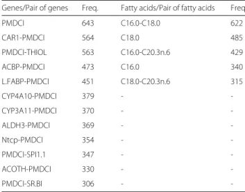
To account for interactions between features into our model, we calculated pair-wise kernels for nutrigenomic data. Although the number of sub-kernels was huge (120+ 120×119/2 = 7260 sub-kernels for genes, 21+21× 20/2 = 231 sub-kernels for fatty acids), TSKCCA suc-cessfully extracted a significant association (p < 0.001 using a permutation test). To evaluate the stability of fea-ture selection, we performed TSKCCA on 1000 runs with data generated by random sampling of empirical data with replacement. Table 3 shows the frequencies of features (i.e. pairs of features) selected across 1000 runs, sug-gesting thatPMDCI played an important role within the interactions.
Discussion
Other researchers have employed the sparse additive model [13] to extend KCCA to high-dimensional prob-lems, and have defined two equivalent formulations, such as sparse additive functional CCA (SAFCCA) and sparse additive kernel CCA (SAKCCA) [12]. The former was defined in a second order Sobolev space and solved using the biconvex back-fitting procedure. The latter, defined in RKHS, was derived by applying representer theorem to the former. Given some function fm ∈ Hm, these algorithms optimize the additive model, f1 ∈ H1,f2 ∈ H2,. . .,fp∈Hp. In contrast, our formulation supposes an additive kernel, such asηmKm associated with RKHS Hadd and finds correlations in this space. This approach enables us to reveal multiple components of associations.
Fig. 5Feature selection of sparse CCA in nutrigenomic data.Leftandright panelsshow selected genes and fatty acids, respectively. Genes marked
Fig. 6Feature selection of TSKCCA using nutrigenomic data.Leftandright panelsshow selected genes and fatty acids, respectively. Genes marked with asterisks show significantly different expression in different genotypes. The left panel shows that the 1st singular vector extracts nonlinear correlations associated with the genotype
Some problems specific to KCCA, such as choosing two parameters (i.e. regularization parameterκand the width parameter γ) and the number of components, remain unsolved. While cross validation is applicable to set these values [24], they are fixed for simplicity in our study, based on the previous study [9].
Next, we discuss the validity of feature selection in nutrigenomic data performed using sparse CCA and TSKCCA. In the original study, the authors focused on the role of PPARαas a major transcriptional regulator of lipid metabolism and determined that PPARα regulates the expression of many genes in mouse liver under lower dietary fat conditions [22]. They provided a list of genes that have significantly different expression levels between wild-type and PPARα-deficient mice. While only a few genes selected by sparse CCA were included in the list, 13 out of 14 genes selected with the 1st singular vector in TSKCCA were included in the list. This result shows
that TSKCCA successfully extracts meaningful nonlinear associations induced by PPARα-deficiency.
Moreover, in our analysis of pair-wise kernels, most of the frequently selected pairs of genes retained PMDCI known as a sort of enoyl-CoA isomerases involved inβ -oxidation of polyunsaturated fatty acids. This implies that the interactions ofPMDCI and other genes contribute to lipid metabolism in PPARα-deficient mice.
Many variants of sub-kernels, such as string kernels or graph kernels, can be employed in the same framework. In the field of bioinformatics, Yamanishi et al. adopted integrated KCCA (IKCCA), which exploited the simple sum of multiple kernels to combine many sorts of bio-logical data [11]. This technique can be improved by optimizing weight coefficients of each kernel in the frame of TSKCCA. Finally, if kernels are defined on groups of features, it enables us to perform group-wise feature selec-tion, just like group sparse CCA [25–27]. It is beneficial
Fig. 7Box plot of test correlations in nutrigenomic data.Leftandright panelsshow the box plot of 100 times test correlation using sparse CCA and
Table 3Frequency of selection per sub-kernel corresponding to genes (left) and fatty acids (right) in nutrigenomic data
Genes/Pair of genes Freq. Fatty acids/Pair of fatty acids Freq
PMDCI 643 C16.0-C18.0 622 CAR1-PMDCI 564 C18.0 485 PMDCI-THIOL 563 C16.0-C20.3n.6 429 ACBP-PMDCI 473 C16.0 340 L.FABP-PMDCI 451 C18.0-C20.3n.6 315 CYP4A10-PMDCI 379 - -CYP3A11-PMDCI 370 - -ALDH3-PMDCI 369 - -Ntcp-PMDCI 354 - -PMDCI-SPI1.1 347 - -ACOTH-PMDCI 330 - -PMDCI-SR.BI 306 -
-to consider group-wise feature selection for biomarker detection problems.
Conclusions
This paper proposes a novel extension of kernel CCA that we call two-stage kernel CCA, which is able to identify multiple canonical variables from sparse features. This method optimizes the sparse weight coefficients of pre-specified sub-kernels as a sparse matrix decomposition before performing standard kernel CCA. This procedure enables us to achieve interpretability by removing irrel-evant features in the context of nonlinear correlational analysis.
Through three numerical experiments, we have demon-strated that TSKCCA is more useful for higher dimen-sional data and for extracting multiple nonlinear associa-tions than an existing method, SAFCCA. Using nutrige-nomic data, our results show that TSKCCA can retrieve information about genotype and may reveal an interactive mechanism of lipid metabolism in PPARα-deficient mice.
Endnotes
1In this article, [·]
nn denotes the(n,n)-th elements of the matrix enclosed by the brackets.
2In this article,x
.mdenotes them-th feature ofx. Abbreviations
CCA: Canonical correlation analysis; HSIC: Hilbert-Schmidt independent criterion; KCCA: Kernel canonical correlation analysis; MKL: Multiple kernel learning; RKHS: Reproducing kernel Hilbert space; SAFCCA: Sparse additive functional canonical correlation analysis; TSKCCA: Two-stage kernel canonical correlation analysis
Acknowledgements
We thank Dr. Mitsuo Kawato, Dr. Noriaki Yahata, and Dr. Jun Morimoto for their valuable comments, and Dr. Steven D. Aird for editing the manuscript.
Funding
This work was supported by a Grant-in-Aid for Scientific Research on Innovative Areas: Artificial Intelligence and Brain Science (16H06563), the Strategic Research Program for Brain Sciences from Japan Agency for Medical Research and Development, AMED, and Okinawa Institute of Science and Technology Graduate University.
Availability of data and materials
The datasets analyzed during the current study are available from https://cran. r-project.org/web/packages/CCA.
Our code for TSKCCA and synthetic data is available in https://github.com/ kosyoshida/TSKCCA.
Authors’ contributions
KY designed the model and developed the algorithm. KY, JY, and KD participated in writing of the manuscript. All authors read and approved the final manuscript.
Competing interests
The authors declare that they have no competing interests. Consent for publication
Not applicable.
Ethics approval and consent to participate Not applicable.
Author details
1Graduate School of Informatics, Kyoto University, Kyoto, Japan.2Neural
Computation Unit, Okinawa Institute of Science and Technology, Okinawa, Japan.3Graduate School of Information Science, Nara Institute of Science and
Technology, Nara, Japan.
Received: 14 October 2016 Accepted: 8 February 2017
References
1. Hotelling H. Relations between two sets of variates. Biometrika. 1936;28: 321–77.
2. Yamanishi Y, Vert JP, Kanehisa M. Protein network inference from multiple genomic data: a supervised approach. Bioinformatics. 2004;20(suppl 1):363–70.
3. Waaijenborg S, Verselewel de Witt Hamer PC, Zwinderman AH. Quantifying the association between gene expressions and dna-markers by penalized canonical correlation analysis. Stat Appl Genet Mol Biol. 2008;7(1):3.
4. Witten DM, Tibshirani R, Hastie T. A penalized matrix decomposition, with applications to sparse principal components and canonical correlation analysis. Biostatistics. 2009;10(3):515–34.
5. González I, Déjean S, Martin PG, Gonçalves O, Besse P, Baccini A. Highlighting relationships between heterogeneous biological data through graphical displays based on regularized canonical correlation analysis. J Biol Syst. 2009;17(02):173–99.
6. Wilms I, Croux C. Sparse canonical correlation analysis from a predictive point of view. Biom J. 2015;57(5):834–51.
7. Parkhomenko E, Tritchler D, Beyene J, et al. Sparse canonical correlation analysis with application to genomic data integration. Stat Appl Genet Mol Biol. 2009;8(1):1–34.
8. Akaho S. A kernel method for canonical correlation analysis. In: Proceedings of the International Meeting of the Psychometric Society (IMPS2001). Osaka: Springer Japan; 2001.
9. Bach FR, Jordan MI. Kernel independent component analysis. J Mach Learn Res. 2003;3:1–48.
10. Vert JP, Kanehisa M. Graph-driven feature extraction from microarray data using diffusion kernels and kernel cca. In: Advances in Neural Information Processing Systems. Vancouver: NIPS Foundation; 2002. p. 1425–432. 11. Yamanishi Y, Vert JP, Nakaya A, Kanehisa M. Extraction of correlated
gene clusters from multiple genomic data by generalized kernel canonical correlation analysis. Bioinformatics. 2003;19(suppl 1):323–30. 12. Balakrishnan S, Puniyani K, Lafferty JD. Sparse additive functional and
Machine Learning, ICML 2012, Edinburgh, Scotland, UK, June 26 - July 1, 2012. The International Machine Learning Society; 2012.
13. Ravikumar P, Lafferty J, Liu H, Wasserman L. Sparse additive models. J R Stat Soc Ser B Stat Methodol. 2009;71(5):1009–30.
14. Gretton A, Bousquet O, Smola AJ, Schölkopf B. Measuring statistical dependence with hilbert-schmidt norms. In: Algorithmic Learning Theory, 16th International Conference, ALT 2005, Singapore, October 8-11, 2005, Proceedings. Springer; 2005. p. 63–77.
15. Cristianini N, Shawe-taylor J, Elisseeff A, Kandola J. On kernel-target alignment. In: Advances in Neural Information Processing Systems 14. Vancouver; 2001. Citeseer.
16. Chang B, Krüger U, Kustra R, Zhang J. Canonical correlation analysis based on hilbert-schmidt independence criterion and centered kernel target alignment. In: Proceedings of the 30th International Conference on Machine Learning, ICML 2013, Atlanta, GA, USA, 16-21 June 2013. The International Machine Learning Society; 2013. p. 316–24.
17. Lanckriet GR, Cristianini N, Bartlett P, Ghaoui LE, Jordan MI. Learning the kernel matrix with semidefinite programming. J Mach Learn Res. 2004;5: 27–72.
18. Bach FR, Lanckriet GR, Jordan MI. Multiple kernel learning, conic duality, and the smo algorithm. In: Proceedings of the Twenty-first International Conference on Machine Learning. ACM; 2004. p. 6.
19. Cortes C, Mohri M, Rostamizadeh A. Two-stage learning kernel algorithms. In: Proceedings of the 27th International Conference on Machine Learning (ICML-10), June 21-24, 2010, Haifa, Israel. The International Machine Learning Society; 2010. p. 239–46. 20. Yamada M, Jitkrittum W, Sigal L, Xing EP, Sugiyama M.
High-dimensional feature selection by feature-wise kernelized lasso. Neural Comput. 2014;26(1):185–207.
21. Kloft M, Brefeld U, Sonnenburg S, Zien A. Lp-norm multiple kernel learning. J Mach Learn Res. 2011;12:953–97.
22. Martin P, Guillou H, Lasserre F, Déjean S, Lan A, Pascussi J, Sancristobal M, Legrand P, Besse P, Pineau T. Novel aspects of pparalpha-mediated regulation of lipid and xenobiotic metabolism revealed through a nutrigenomic study. Hepatol (Baltim Md.) 2007;45(3):767–77. 23. González I, Déjean S, Martin PG, Baccini A, et al. Cca: An r package to
extend canonical correlation analysis. J Stat Softw. 2008;23(12):1–14. 24. Leurgans SE, Moyeed RA, Silverman BW. Canonical correlation analysis
when the data are curves. R Stat Soc Ser B Methodol, J. 1993;725–40. 25. Yuan M, Lin Y. Model selection and estimation in regression with
grouped variables. J R Stat Soc Ser B Methodol. 2006;68(1):49–67. 26. Bach FR. Consistency of the group lasso and multiple kernel learning. J
Mach Learn Res. 2008;9:1179–225.
27. Lin D, Zhang J, Li J, Calhoun VD, Deng HW, Wang YP. Group sparse canonical correlation analysis for genomic data integration. BMC Bioinforma. 2013;14(1):245.
• We accept pre-submission inquiries
• Our selector tool helps you to find the most relevant journal
• We provide round the clock customer support
• Convenient online submission
• Thorough peer review
• Inclusion in PubMed and all major indexing services
• Maximum visibility for your research Submit your manuscript at
www.biomedcentral.com/submit