FEATURE SELECTION BASED ON SEQUENTIAL
ORTHOGONAL SEARCH STRATEGY
By
Azlyna Senawi
A thesis submitted to the University of Sheffield
for the degree of
Doctor of Philosophy
Department of Automatic Control & Systems Engineering
The University of Sheffield
Mappin Street
Sheffield S1 3JD
United Kingdom
To Nafrizuan, my amazing husband, and the apples of my eyes; Ismael, Ielyas and Iedris.
To the memory of Abah,
I
Abstract
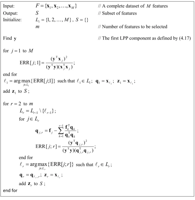
This thesis introduces three new feature selection methods based on sequential orthogonal search strategy that addresses three different contexts of feature selection problem being considered. The first method is a supervised feature selection called the maximum relevance–minimum multicollinearity (MRmMC), which can overcome some shortcomings associated with existing methods that apply the same form of feature selection criterion, especially those that are based on mutual information. In the proposed method, relevant features are measured by correlation characteristics based on conditional variance while redundancy elimination is achieved according to multiple correlation assessment using an orthogonal projection scheme. The second method is an unsupervised feature selection based on Locality Preserving Projection (LPP), which is incorporated in a sequential orthogonal search (SOS) strategy. Locality preserving criterion has been proved a successful measure to evaluate feature importance in many feature selection methods but most of which ignore feature correlation and this means these methods ignore redundant features. This problem has motivated the introduction of the second method that evaluates feature importance jointly rather than individually. In the method, the first LPP component which contains the information of local largest structure (LLS) is utilized as a reference variable to guide the search for significant features. This method is referred to as sequential orthogonal search for local largest structure (SOS-LLS). The third method is also an unsupervised feature selection with essentially the same SOS strategy but it is specifically designed to be robust on noisy data. As limited work has been reported concerning feature selection in the presence of attribute noise, the third method is thus attempts to make an effort towards this scarcity by further exploring the second proposed method. The third method is designed to deal with attribute noise in the search for significant features, and kernel pre-images (KPI) based on kernel PCA are used in the third method to replace the role of the first LPP component as the reference variable used in the second method. This feature selection scheme is referred to as sequential orthogonal search for kernel pre-images (SOS-KPI) method. The performance of these three feature selection methods are demonstrated based on some comprehensive analysis on public real datasets of different characteristics and comparative studies with a number of state-of-the-art methods. Results show that each of the proposed methods has the capacity to select more efficient feature subsets than the other feature selection methods in the comparative studies.
II
Acknowledgement
In the name of God, the Most Gracious, the Most Merciful.
First and foremost, all praises and thanks are due to the Almighty Allah, the Lord of the Universe, who generously gave me the strength, knowledge and opportunity to complete this PhD journey. No word could adequately describe my upmost gratitude for His innumerable favours showered upon me along the way.
I am greatly indebted to my supervisor, Dr. Hua Liang Wei, whose professional guidance, thoughtful consideration and steady support over the years have been invaluable. Without his involvement, intellectual advice and critical comments, this thesis would not have been possible. Thanks to him for being receptive to my ideas and I consider the granted scientific freedom during the course of my study as a positive learning experience.
I am also indebted to Professor Billings as my second supervisor, who took time out of his busy schedule to give constructive feedbacks and helpful suggestions for the research work. I would like to gratefully acknowledge Malaysian Government and Universiti Malaysia Pahang for the scholarship award under Skim Latihan Akademik IPTA (SLAI) program that kept me financially sound throughout a three-and-a-half year study period.
A heartfelt thanks to all my friends who made my Sheffield experience memorable and special, in particular, Vicktor, Ain, Nana, Ruzaini, Abang Zack, Kak Niza, Maniha, Hyreil and Zhang Yang. Personally, I would like to thank Kak Anoi and Abang Zam for their kind helps and countless delicious meals delivered to our doorstep at Basford Street.
A bunch of thanks is reserved to my friends, Fizah, Rozieana and Najihah, not only for helping me in many ways but also for lending an ear for my sad stories since I came back to Malaysia and need to finish my PhD from far.
My sincere thanks and deepest appreciation go to my late dad (Abah) and mum for their emotional support and unwavering faith in me although they don’t understand what I researched on. Abah, I never realized how much I love you till you left me during the final stage of my thesis write-up. I really wish you were around to witness your dream come true. My sincere thanks are extended to my parents in law for their love, care and prayers through all these years.
III My greatest gratitude to my dearest husband, Nafrizuan, for making things keep going on even at the hardest of times. During the last six months of writing this thesis I was particularly preoccupied but he always try to make the process as easy as possible for me. I cannot express how much thankful I am for his unremitting patience and support from the moment we began the PhD journey together at ACSE. Certainly, this thesis would not have been in its present form without him.
The last word goes for my three little sons: Ismael, Ielyas and Iedris, to whom I owe lots of fun hours. They have been the light of my life and always been my constant source of strength to get this roller coaster journey through to the end.
IV
Table of Contents
ABSTRACT…………. ... I ACKNOWLEDGEMENT ... II TABLE OF CONTENTS ... IV LIST OF ABBREVIATIONS ... VIII LIST OF FIGURES ... IX LIST OF TABLES ... XI CHAPTER 1 INTRODUCTION ... 1 1.1 Introduction ... 1 1.2 Motivation ... 1 1.3 Research Objectives ... 11
1.4 Research Contributions and Publications ... 12
1.5 Organization of the Thesis ... 13
1.6 Summary ... 14
CHAPTER 2 FEATURE SELECTION AND FORWARD ORTHOGONAL SEARCH ... 15
2.1 Introduction ... 15
2.2 Feature Selection Objectives ... 15
V
2.4 Feature Subset Generation ... 17
2.4.1 Search Starting Point... 17
2.4.2 Search Strategy ... 17
2.5 Feature Subset Evaluation Criteria ... 20
2.6 Feature Selection Models ... 21
2.6.1 Filter Model ... 21
2.6.2 Wrapper Model ... 22
2.6.3 Hybrid Model ... 22
2.7 Supervised and Unsupervised Feature Selection ... 23
2.8 Orthogonal Transformation ... 24
2.9 Summary ... 25
CHAPTER 3 A NEW RELEVANCY-REDUNDANCY METHOD FOR FEATURE SELECTION AND RANKING ... 26
3.1 Introduction ... 26
3.2 Relevancy and Redundancy ... 27
3.3 Related Work ... 27
3.4 Feature Relevancy Assessment ... 29
3.5 Multicollinearity Redundancy and the Squared Multiple Correlation Coefficient ... 33
3.5.1 Multicollinearity Redundancy ... 33
3.5.2 The Squared Multiple Correlation Coefficient ... 34
3.6 Monitoring Criterion ... 35
VI
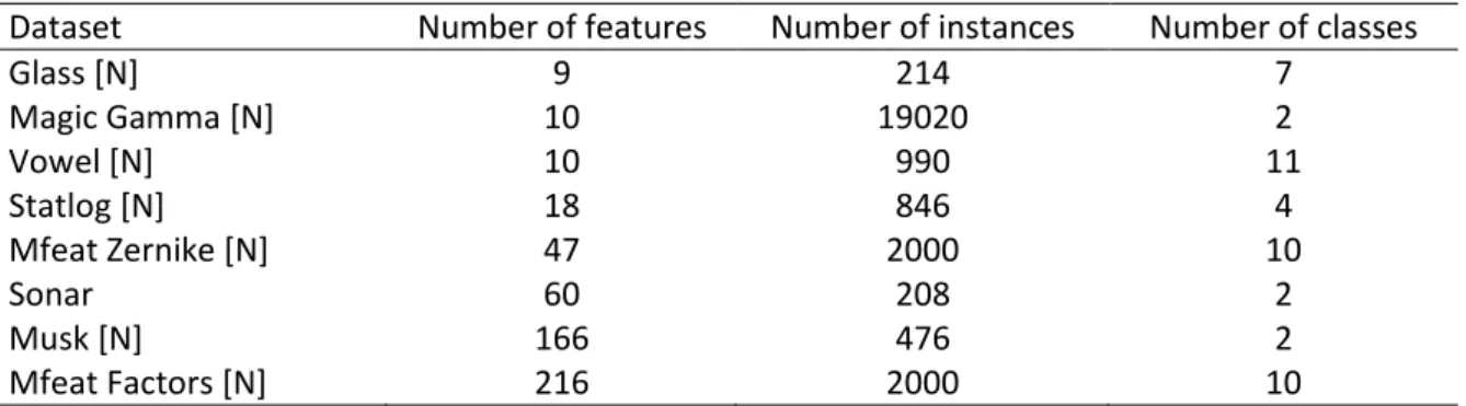
3.7.1 Benchmark Datasets... 38
3.7.2 Comparison with Similar Methods ... 38
3.7.3 Validation Classifiers ... 39
3.7.4 Cross Validation Procedure ... 39
3.8 Numerical Results and Discussion ... 39
3.9 Summary ... 54
CHAPTER 4 UNSUPERVISED FEATURE SELECTION BASED ON LOCAL LARGEST STRUCTURE ... 55
4.1 Introduction ... 55
4.2 Related Work ... 55
4.2.1 Locality Preserving Projection ... 55
4.2.2 Laplacian Score ... 59
4.2.3 Multi-Cluster Feature Selection ... 60
4.2.4 Minimum-Maximum Laplacian Score (MMLS) ... 61
4.3 The Proposed Algorithm for Feature Ranking and Selection ... 63
4.4 Experimental Setup and Evaluation ... 69
4.4.1 First Category of Benchmark Datasets ... 70
4.4.2 Second Category of Benchmark Datasets ... 73
4.5 Summary ... 80
CHAPTER 5 FEATURE SELECTION BASED ON KERNEL PRE-IMAGES ... 81
VII
5.2 Kernel PCA and the Pre-Image Problem ... 81
5.3 Feature Selection Based on Pre-Images of Kernel PCA ... 84
5.4 Monitoring Criterion and Search Procedure ... 86
5.5 Experimental Setup and Procedure ... 90
5.5.1 Modified Benchmark Datasets ... 90
5.5.2 Comparison with Other Methods ... 92
5.5.3 Validation Classifiers ... 92
5.5.4 Cross-Validation Procedure ... 92
5.6 Numerical Results and Discussion ... 93
5.7 Summary ... 100
CHAPTER 6 CONCLUSION ... 102
6.1 Research Summary and Conclusion ... 102
6.2 Future Direction of the Research ... 104
VIII
List of Abbreviations
CART : Classification and regression trees
FOS-MOD : Forward orthogonal search by maximizing the overall dependency
k-NN : k-nearest neighbour
LDA : Linear discriminant analysis LPP : Locality preserving projection LS : Laplacian score
MCFS : Multi-cluster feature selection
MIFS : Mutual information based feature selection MMLS : Minimum-maximum Laplacian score
MRmMC : Maximum relevance-minimum multicollinearity mRMR : Minimal-redundancy-maximal-relevance PCA : Principal component analysis
SOS-KPI : Sequential orthogonal search of kernel pre-images SOS-LLS : Sequential orthogonal search for local largest structure SVM : Support vector machine
IX
List of Figures
Figure 1.1: Nine Technological Pillars of Industrial Revolution 4.0 (Gerbert, et al., 2015).. .... 2
Figure 2.1: Four basic steps of a feature selection method (Dash & Liu, 2003). ... 16
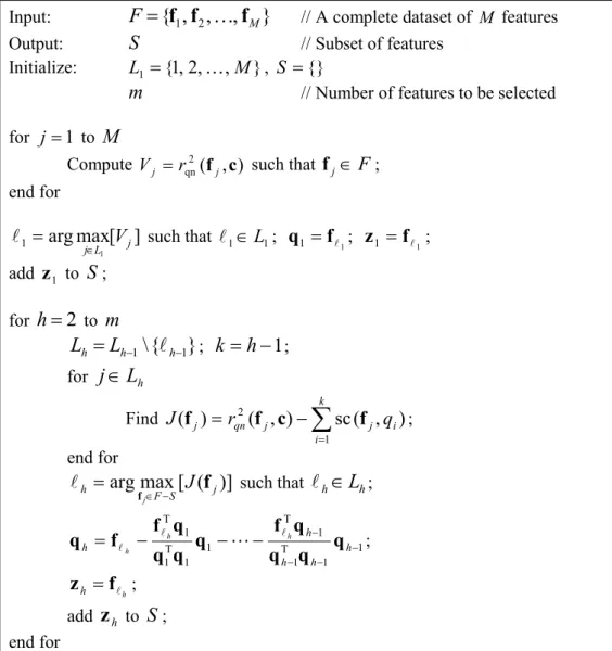
Figure 3.1: The MRmMC algorithm... 37
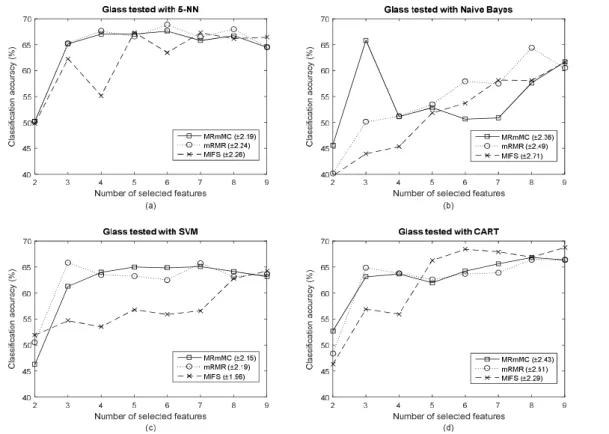
Figure 3.2: Classification results for Glass dataset over different number of selected features,
tested with four classifiers: (a) 5-NN, (b) Naïve Bayes, (c) SVM and (d) CART. Each plot shows comparison among MRmMC, mRMR and MIFS methods. ... 40
Figure 3.3: Classification results for Magic Gamma dataset over different number of selected
features, tested with four classifiers: (a) 5-NN, (b) Naïve Bayes, (c) SVM and (d) CART. Each plot shows comparison among MRmMC, mRMR and MIFS methods. ... 41
Figure 3.4: Classification results for Vowel dataset over different number of selected features,
tested with four classifiers: (a) 5-NN, (b) Naïve Bayes, (c) SVM and (d) CART. Each plot shows comparison among MRmMC, mRMR and MIFS methods. ... 42
Figure 3.5: Classification results for Statlog dataset over different number of selected features,
tested with four classifiers: (a) 5-NN, (b) Naïve Bayes, (c) SVM and (d) CART. Each plot shows comparison among MRmMC, mRMR and MIFS methods. ... 43
Figure 3.6: Classification results for Mfeat Zernike dataset over different number of selected
features, tested with four classifiers: (a) 5-NN, (b) Naïve Bayes, (c) SVM and (d) CART. Each plot shows comparison among MRmMC, mRMR and MIFS methods. ... 44
Figure 3.7: Classification results for Sonar dataset over different number of selected features,
tested with four classifiers: (a) 5-NN, (b) Naïve Bayes, (c) SVM and (d) CART. Each plot shows comparison among MRmMC, mRMR and MIFS methods. ... 45
Figure 3.8: Classification results for Musk dataset over different number of selected features,
tested with four classifiers: (a) 5-NN, (b) Naïve Bayes, (c) SVM and (d) CART. Each plot shows comparison among MRmMC, mRMR and MIFS methods. ... 46
X
Figure 3.9: Classification results for Mfeat Factors dataset over different number of selected
features, tested with four classifiers: (a) 5-NN, (b) Naïve Bayes, (c) SVM and (d) CART. Each plot shows comparison among MRmMC, mRMR and MIFS methods. ... 47
Figure 4.1: PC1-PC2 score plot for the Alate Adelges dataset based on (a) full feature set, (b)
the first four selected features and (c) the first five selected features. ... 71
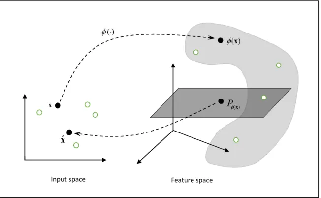
Figure 5.1: Pre-image problem in kernel PCA. ... 83
Figure 5.2: Comparison of the total win/tie/loss counts of the SOS-KPI method versus other
XI
List of Tables
Table 2.1: A comparison of different search strategies. ... 20
Table 3.1: A summary of the datasets characteristics. ... 38
Table 3.2: A comparison of the average classification accuracy based on the first m selected
features. ... 49
Table 3.3: A comparison of the average classification accuracy based on the first m selected
features. ... 50
Table 3.4: The least number of selected features, , by MRmMC, mRMR and MIFS
methods that gives classification accuracy close to (at most 5% less than the full set accuracy) or better than the full feature set. The symbol “•” (or “□”) denotes the proposed method has lower (or larger) value of mleast than the compared method. Results are based on Glass, Magic Gamma, Vowel and Statlog datasets. ... 52
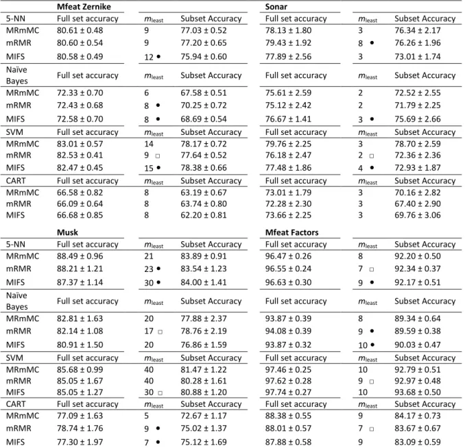
Table 3.5: The least number of selected features, mleast, by MRmMC, mRMR and MIFS
methods that gives classification accuracy close to (at most 5% less than the full set accuracy) or better than the full feature set. The symbol “•” (or “□”) denotes the proposed method has lower (or larger) value of mleast than the compared method. Results are based on Mfeat Zernike, Sonar, Musk and Mfeat Factors datasets. ... 53
Table 3.6: A comparison of win/tie/loss counts of the MRmMC method against the other
methods. The counts are based on the results presented in Table 3.4 and Table 3.5... 53
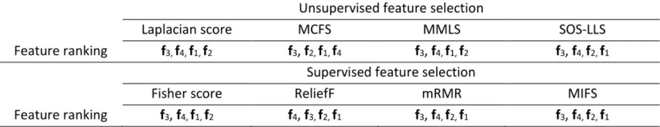
Table 4.1: Feature ranking results of the Iris dataset given by different feature selection methods.
... 73
Table 4.2: Important details of the used benchmark datasets for 2nd category. ... 73
Table 4.3: Performance comparison of the average classification accuracy based on m selected
features with four classifiers. The value within the bracket is the p-value to test whether the accuracy of SOS-LLS is significantly larger than that obtained by its competitor. ... 76
XII
Table 4.4: Performance comparison of the average classification accuracy based on m selected
features with four classifiers. The value within the bracket is the p-value to test whether the accuracy of SOS-LLS is significantly larger than that obtained by its competitor. ... 77
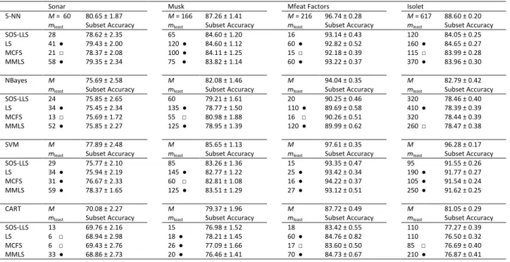
Table 4.5: The least feature subset size, mleast, given by different feature selection methods that
reach classification accuracy close to (with tolerance no more than 5% less) or maybe more than that obtained by the full feature set of size M. The symbol “●” (or “□”) marks that SOS-LLS gives smaller (or larger) value of mleast than the compared method. Results are based on eight benchmarks datasets... 78
Table 4.6: The least feature subset size, mleast, given by different feature selection methods that
reach classification accuracy close to (with tolerance no more than 5% less) or maybe more than that obtained by the full feature set of size M. The symbol “●” (or “□”) marks that SOS-LLS gives smaller (or larger) value of mleast than the compared method. Results are based on four benchmarks datasets... 79
Table 4.7: Tabulations of the win/tie/loss counts of the SOS-LLS method versus other methods.
The counts are based on the results presented in Table 4.5 and Table 4.6. ... 79
Table 5.1: Characteristics of the used benchmark datasets. ... 91
Table 5.2: The least number of selected features, mleast, induced by SOS-KPI, LS, MCFS and
MMLS methods that gives classification accuracy close to (at most 5% less than the full set accuracy) or better than the full feature set. The symbol “●” (or “□”) denotes the proposed method has lower (or larger) value of mleast than the compared method. Results are based on Pima Diabetes, Glass and Vowel datasets... 95
Table 5.3: The least number of selected features, mleast, induced by SOS-KPI, LS, MCFS and
MMLS methods that gives classification accuracy close to (at most 5% less than the full set accuracy) or better than the full feature set. The symbol “●” (or “□”) denotes the proposed method has lower (or larger) value of mleast than the compared method. Results are based on Statlog, Wdbc and Ionosphere datasets. ... 96
XIII
Table 5.4: The least number of selected features, mleast, induced by SOS-KPI, LS, MCFS and
MMLS methods that gives classification accuracy close to (at most 5% less than the full set accuracy) or better than the full feature set. The symbol “●” (or “□”) denotes the proposed method has lower (or larger) value of mleast than the compared method. Results are based on Waveform, Mfeat Zernike and Sonar datasets. ... 97
Table 5.5: The least number of selected features, mleast, induced by SOS-KPI, LS, MCFS and
MMLS methods that gives classification accuracy close to (at most 5% less than the full set accuracy) or better than the full feature set. The symbol “●” (or “□”) denotes the proposed method has lower (or larger) value of mleast than the compared method. Results are based on Musk, Mfeat Factors and Isolet datasets. ... 98
Table 5.6: A comparison of the win/tie/loss counts of the SOS-KPI method against other
methods for different categories of dimensional size. The counts are based on the results presented in Table 5.2 through Table 5.5 when the datasets are corrupted with 10% of attribute noise and considering all four classifiers. ... 99
Table 5.7: A comparison of the win/tie/loss counts of the SOS-KPI method against other
methods for different categories of dimensional size. The counts are based on the results presented in Table 5.2 through Table 5.5 when the datasets are corrupted with 20% of attribute noise and considering all four classifiers. ... 99
Table 5.8: A comparison of the win/tie/loss counts of the SOS-KPI method against other
methods. The counts are based on the results presented in Table 5.2 through Table 5.5 when the datasets are corrupted with 10% attribute noise. ... 100
Table 5.9: A comparison of the win/tie/loss counts of the SOS-KPI method against other
methods. The counts are based on the results presented in Table 5.2 through Table 5.5 when the datasets are corrupted with 20% attribute noise. ... 100
1
Chapter 1
Introduction
1.1
Introduction
This chapter presents an overview of the research conducted. It starts with a discussion of the motivation of the research to highlight the research problems. Then, objectives of this research are established. This chapter also allocates a section to preview the contribution of the research to the world of knowledge. The publications as outcomes of the research also have been listed. This chapter ends with a description of the overall thesis organisation.
1.2
Motivation
The birth of the Industrial Revolution has brought forward technological advances to the world and has thus motivated the industrial productivity to growth vividly (Gerbert, et al., 2015). As the world is currently moving towards the fourth wave of technological advancement, digital industrial technology has become the main essence and attracted considerable attention in recent years from numerous parties including policy-makers, practitioners, research communities as well as government organisations. This era is penned as Industrial Revolution 4.0 (Gerbert, et al., 2015) which is often simply noted as Industry 4.0. The route to the Industry 4.0 has been focused on nine foundational technology advances, more specifically referred as Industry 4.0 Technology Pillars as shown in Figure 1.1.
Notice that one of the pillars is “big data and analytics”. The two key components, big data and analytic, that become the basis for the pillar are really two different things but they are intertwined. As the two teamed up and worked together, they then brought a new discipline known as big data analytics that is increasingly becoming a trending practice by many organisations with a primary goal to gain useful information from big data (Sivarajah, et al., 2017). The potential of big data is evident from the fact that among the highest paid jobs in the
2 world are related to big data (Bennett, 2017). According to a Glassdoor report, data scientist career was ranked as the number one best job in the United States for 2018, meanwhile it is the sixth best job in the UK in 2017 (Glassdoor Inc., 2018). Because there are still enormous sets of untapped big data in the industrial world, they thus offer valuable information with many new opportunities that are beneficial in aiding practitioners to have sound understanding about certain activities or processes. According to O'Donovan et al. (2015), big data analytics will provide significant help to the industrial community to optimize the quality of a production, perform better operations, acquire excellent services and most importantly support accurate and timely decision-making.
Figure 1.1: Nine Technological Pillars of Industrial Revolution 4.0 (Gerbert, et al., 2015).
Big data stored in any information system including but not limited to industrial related databases require special methods for processing and analysing before the data can be used to assist decision making. Under such a circumstance, there is a demand to automate the process intelligently and use each massive dataset as a source to extract useful information (Bhadani & Jothimani, 2016). Among the tools that can be utilized to meet the requirement is data mining.
Data mining can be defined as a process of discovering useful patterns from a large amount of data (Witten & Frank, 2005). It has been applied successfully in many different fields such as retail industry, marketing, banking, healthcare, science and engineering.
3 However, mining scientific data is often different from mining business or commercial data. According to Sivarajah et al. (2017), data analysis problems for science and engineering fields are more complex and therefore require more specific solutions. Hence, special attention must be given to the unique requirements of scientific datasets and related issues need to be addressed accordingly.
One of the most complex natures that receive considerable attention among researchers is the explosive growth in sizes of datasets with millions to billions of records. Remarkable innovation and advancement in data storage have made collecting and saving such tremendous amount of data more feasible. While massive datasets can be utilized as a source to mine interesting information, the analysis accuracy and efficiency could become intractable due to the high dimensionality. Although there are methods that can be used to construct predictive models from high dimensional data with high accuracy (Breiman, 2001), data analysis in lower dimensional space is still desirable in many applications since modelling high dimensional data is more likely too computationally expensive. In many applications, the analysis of big data can be performed in a reduced dimensional space and the resulting performance can be even better than that obtained from using the original datasets (Zhang, et al., 2009; Wang, et al., 2012; Likitjarernkul, et al., 2017) because the original feature space may contain a large number of irrelevant and redundant features. Hence, it is desirable and sometimes crucial to identify and remove these insignificant features so that learning from data become technically more effective. This can be done via dimensionality reduction which can be achieved by two different strategies, namely, feature extraction and feature selection.
In feature extraction approaches such as principal component analysis (Wold, et al., 1987) and linear discriminant analysis (Balakrishnama & Ganapathiraju, 1998), new features are constructed from the original features to form a new reduced dimensional space by combining or transforming the original features using some functional mapping. Although the new features in the new reduced dimensional space are related to the original features, the actual interpretation of the original features and hence the relation to the original system variables is completely lost in most cases. This drawback should be taken into account when considering dimensionality reduction since the actual interpretation may be important to understand the learning process that generates the new feature space (Somol, 2010). Feature extraction also often associated with computational inefficiency despite the fact that it may significantly reduce dimensional space since the new constructed features are based on
4 transformation that involves all original features including irrelevant and redundant features. Nevertheless, its main advantage over feature selection is in the fact that no information from the original features is wasted or lost in the dimensionality reduction process (Yang, et al., 2010). This fact further offers another advantage of feature extraction approach in that the reduced dimensional space, in general, have more compact representation of the original features than the feature selection approach (Gao, et al., 2017).
Unlike feature extraction which attempts to create new features based on all original features, feature selection is an approach which requires a selection of the most significant subset of features to a targeted concept by removing redundant and irrelevant features (Wei & Billings, 2007). These redundant and irrelevant features can be ignored because they give very little or no unique information for data analysis and modelling (Hira & Gilles, 2015). Moreover, in many cases, the presence of irrelevant and redundant features can only make data analysis and modelling more complicated without increasing accuracy. Since feature selection does not alter the actual interpretation of any feature involve, it has the advantage of being able to facilitate the understanding of what really generates the new feature space and significantly benefit future analysis. Commonly used feature selection methods include Fisher score (Jaakkola & Haussler, 1999), Relief (Kira & Rendell, 1992), minimal-redundancy-maximal-relevance (mRMR) (Peng, et al., 2005) and Laplacian score (He, et al., 2006), to name a few. In contrast to feature extraction, the feature selection approachis perceived as having a lower flexibility in finding a reduced feature space, particularly when the best low-dimensional feature set for a certain data mining task should not only consists of original features (Zhang, et al., 2008).
Much of the early work on feature selection focused on choosing relevant features. But later, when the existence and effect of redundant features have been discovered, many have been directed to deal with both relevant and redundant features in the selection process. Feature redundancy was defined in some explicit or inexplicit manner, highlighting the need to remove redundant features (John, Kohavi, & Pfleger, 1994; Pudil, Novovicova, & Kittler, 1994; Koller & Sahami, 1996; Kohavi & John, 1997; Hall, 1999). For example, in Koller & Sahami (1996), the Markov Blanket filtering process was utilized to form the definition which highlights that a redundant feature removed earlier remains redundant when other features are removed. A more concrete definition of feature redundancy was given in Yu & Liu (2004), which considers
5 an optimal feature subset is the one that essentially contains all strongly relevant features and also weakly relevant but non-redundant features.
The concept of mutual information has been widely employed as an evaluation criterion for choosing a set of relevant and non-redundant features. Some of the most prominent examples include the criteria proposed by Battiti (1994), Kwak & Choi (2002a) and Peng et al. (2005). Mutual information is preferable as an evaluation criterion over the correlation function for many proposed feature selection methods because of its ability to measure arbitrary dependence relationships between two features (Li, 1990; Battiti, 1994). The method is not only limited to numerical features, but also applies to symbolic features consisting of discrete categories (Li, 1990). These two advantages made the mutual information based criterion to be seen as a more universal and robust measure.
Despite the aforementioned advantages, the mutual information criterion also has a few notable drawbacks. Mutual information computation is straightforward for discrete (categorical) random variables where an exact solution can be obtained easily. However, for continuous random variables which are frequently encountered in mutual information computations, it is difficult to gain the exact solution since the computation of the exact probability density functions (pdfs) is impossible (Kwak & Choi, Input feature selection for classification problems, 2002a). Hence, an estimation of the mutual information is required and different methods can be employed. Among the possible methods are histogram-based (Moddemeijer, 1989; Haeri & Ebadzadeh, 2014; Jain & Murthy, 2016), kernel density estimation (Moon, Rajagopalan, & Lall, 1995), k-nearest neighbour (Kraskov, Stogbauer, & Grassberger, 2004; Gao, Oh, & Viswanath, 2017), Parzen window (Kwak & Choi, Input feature selection by mutual information based on Parzen window, 2002b; He, Zhang, Hao, & Zhang, 2015) B-spline (Daub, Steuer, Selbig, & Kloska, 2004), adaptive partitioning (Fraser & Swinney, 1986; Darbellay & Vajda, 1999); and fuzzy-based (Yu, An, & Hu, 2011; Hancer, Xue, Zhang, Karaboga, & Akay, 2015) approaches. These estimation methods typically involve some pre-set parameters whose optimal values heavily depend on problem characteristics. Parameter settings could possibly be the major source of large estimation errors but still the parameters are often assigned with arbitrary values because there is no clear-cut rule provided (Williams & Li, 2009). In addition, there are so many available options for the mutual estimation calculations. Therefore, the efficiency of a feature selection approach greatly relies on the method applied.
6 A frequently used criterion for dimensionality reduction is to identify features with the highest capability to preserve the manifold structure. Such a criterion has gained widespread attention since in many cases of interest, the recorded data are concentrated around a low dimensional manifold (submanifold) which is embedded in a high dimensional ambient space. The popular methods that use this criterion include principal component analysis (Wold, Esbensen, & Geladi, 1987), linear discriminant analysis (Izenman, 2013; Xanthopoulos, Pardalos, & Trafalis, 2013), Laplacian eigenmap (Belkin & Niyogi, 2003), locally linear embedding (Roweis & Saul, 2000), locality preserving projection (LPP) (He & Niyogi, Locality preserving projections, 2004) and Laplacian score (He, Cai, & Niyogi, Laplacian score in feature selection, 2006). The first two reduce the dimensionality based on global manifold structure preservation while the last four are based on local manifold structure preservation.
The term structure preservation in dimensionality reduction conceptually refers to the scheme to maintain major structural characteristics when mapping the data from high dimensional space to low dimensional space. Technically, the quality of structure preservation can be measured based on the preservation ability in terms of keeping connective similarity among sample points in high dimensional space to sample points in low dimensional representation.
Local structure preservation techniques, as its name implies, emphasize preserving the underlying local structure within the neighbourhood around each data point. Geometrically, such approaches try to retain the nature structure of the close-distance points in the original high dimensional space to a low dimensional representation. While global approaches may also involve preserving local structure, they are different from local techniques in that they attempt to preserve geometric data structure of faraway points in the high dimensional space to a low dimensional space. PCA serves as a good example of global techniques, which is solely based on global structure preservation, while LDA would be a simple example that preserves data structure at both orientations.
PCA is an unsupervised feature extraction approach that aims to find mutually independent projections in the directions where maximum variance of the data lies, which essentially reveals the global manifold structure of the data space. Though this approach may give optimal data representation, it may not be able to provide optimal solution in the classification context. LDA overcomes this problem in supervised mode with the main idea being to find projections that achieve optimum class discrimination in a setting where samples
7 from different classes are well separated as far as possible whereas samples from the same class are scattered together as close as possible. Specifically, these projections are obtained based on an objective function that maximizes the ratio of between-class variance to the within-class variance.
Locality-based structure preservation techniques has gained considerable attention recently and demonstrated to be a successful strategy for dimensionality reduction in many learning tasks such as classification, clustering and visualization. The basic assumption of this technique is based on a simple geometric intuition that two data points tend to share the same characteristic (or class) if they are sufficiently close to each other. This assumption then leads to a key concept that any two close points in the original feature space should remain close in a reduced dimensional space. Owing to the fact that the technique relies on geodesic data structure, a nearest neighbour graph is constructed to model the proximity relation between data points and thereby discovers the intrinsic local manifold structure hidden in the high dimensional space. The technique has the advantage of relatively less affected by outliers since only local distances are considered which helps to prevent overfitting (Belkin & Niyogi, 2003). As data may reside on or close to a nonlinear submanifold structure, various nonlinear locality-based structure preservation methods were suggested in the literature, among which the most popular ones are locally linear embedding (Roweis & Saul, 2000), Isomap (Tenenbaum, De Silva, & Langford, 2000), and Laplacian eigenmap (Belkin & Niyogi, 2003). Though remarkable performance can be achieved by these nonlinear methods, their nonlinear property can only be achieved at the price of high computational cost.
Moreover, these nonlinear methods do not allow any new test point to be mapped into an existing reduced-dimensional space in a straightforward manner. An extension method is therefore required to evaluate the map of a new test point and in this case only estimation of the mapping can be performed (Maaten, Postma, & Herik, 2009). Since error in the estimation may occur, the embedding of new test points may not appropriately reflect the submanifold structure accordingly. Thus, how to map new points into an existing reduced-dimensional space still remains an issue.
Driven by the strength of locality-based geometrical approach as well as the aforementioned nonlinear method deficiencies, LPP emerged to provide a linear version of the Laplacian eigenmap. Although LPP is linear, it shares certain useful common properties of the nonlinear methods due to the fact that LPP adopts the same variational principle as for the
8 Laplacian eigenmap. This enables LPP to discover the nonlinear manifold structure of the data to some extent. Unlike the nonlinear methods that yield mappings which are defined only on training data points, LPP comes with a solution where its mapping is defined everywhere, thereby allows any new test point to be placed naturally into the reduced dimensional space.
Note that all the aforementioned local manifold structure preservation methods (except Laplacian Score) are designed for feature extraction. Yet, these methods have also been applied to feature selection context (Zhao, Lu, & He, 2008; Sun, Todorovic, & Goodison, 2010; Shang, Chang, Jiao, & Xue, 2017; Yao, Liu, Jiang, Han, & Han, 2017). As mentioned earlier, global techniques include either preserving the global structure of data alone or preserving both global and local structures simultaneously. Even so, there has been a growing interest in global manifold structure preservation methods which integrate both global and local information for feature selection. Recently reported studies in this field can be found in Zhang et al. (2011); Ren et al. (2012); Shu et al. (2012); Yu (2012) and Tong & Yan (2014).Interestingly, however, an important discovery made by Liu et al. (2014) revealed that preserving the local structure is more critical than preserving the global structure when feature selection is considered in unsupervised setting.
Real world data are rarely perfect because of numerous reasons such as faulty measuring device, error in data collection, inaccurate source or non-reporting information (e.g. missing data values). All these contributing factors to data imperfection creates a form of data known as noisy data.
Effectively handling noisy data is crucial for a classification task since the presence of noise may severely degrade the predictive accuracy and even slow down the construction of a classifier model (Zhu & Wu, 2004; Saez, Galar, Luengo, & Herrera, Analyzing the presence of noise in multi-class problems: alleviating its influence with the one-vs-one decomposition, 2014; Wickramasinghe, 2017). Such negative impacts on performance usually happen because data corrupted by noise could bring new unnecessary and false-data patterns. For instance, when a high-level noise is present, an additional data cluster is formed or perhaps on the other way round, the extracted pattern will suffer loss of important data clusters (Saez, Galar, Luengo, & Herrera, Analyzing the presence of noise in multi-class problems: alleviating its influence with the one-vs-one decomposition, 2014). Thus, managing noisy data is desired and one feasible solution to this problem is to perform a pre-processing step which specifically aims to enhance the data quality before a classifier is built.
9 In data mining research, there are two categories of noise, namely, class noise and attribute noise (Garcia, Luengo, & Herrera, 2016). Class noise refers to corruptions present in the class attribute which occur when instances are assigned with wrong class labels or when identical instances are recorded with different class labels. Meanwhile, attribute noise refers to errors or corruptions present in one or more values of the input attributes (or features) of the data instances. Generally, managing attribute noise is more complex than class noise. The rationale behind this should be easily understood as attribute noise may distort multiple values of an instance but class noise only corrupt one value, if any. Owing to the same rationale, it is not a good idea to handle noisy data by removing instances containing noise in only some of the attributes while there are still many remaining attributes carrying useful information. In this particular problem, feature selection is seen as an alternative solution to lead the data towards a finer quality.
Since data mining started to gain its popularity in 1990s, feature selection and noisy data have been well studied separately but little is known about the interaction between them. It is only recently that the combination of the two has been empirically investigated. However, among the efforts considering noisy data in feature selection, many have been directed to address the problems of class noise (Altidor, Khoshgoftaar, & Van Hulse, 2011; Shanab, Khoshgoftaar, Wald, & Napolitano, Impact of noise and data sampling on stability of feature ranking techniques for biological datasets, 2012; Shanab, Khoshgoftaar, & Wald, Evaluation of wrapper-based feature selection using hard, moderate, and easy bioinformatics data, 2014; Zhao Z. , 2017) because literature findings have shown that the effect of class noise is more detrimental than attribute noise in the classification context (Quinlan, 1994; Zhu & Wu, 2004; Nettleton, Orriols-Puig, & Fornells, 2010; Saez, Galar, Luengo, & Herrera, Tackling the problem of classification with noisy data using multiple classifier systems: analysis of the performance and robustness, 2013). Despite the fact that class noise is more harmful than the attribute noise, the empirical study conducted by Zhu & Wu (2004) revealed that class noise at some points could be more critical to learning classifiers. While many efforts have been made for dealing with class noise, research on handling attribute noise has not made considerable progress. The report by Zhu & Wu (2004) even highlighted that the class attribute of real-world data, in truth, is typically much cleaner than the input attributes. Accordingly, attribute noise deserves wider attention than it is currently receiving.
10 Over the past few decades, there has been a lot of interest on kernel methods in various learning systems for analysing nonlinear patterns. The basic idea of kernel methods is to map nonlinear data that is linearly inseparable in the original input space to a higher dimensional (possibly infinite) feature space where linear separations (or relations) can be achieved. Since the linear geometry of the data in the feature space is embedded in dot products between data instances, the mapping from the original data space to the feature space does not have to be performed explicitly but just needs some defining form of dot products in the original input space. This nonlinear mapping strategy is the so called ‘kernel trick’, which is the essence of the kernel methods. Taking into advantage of this kernel trick implies that the coordinates of the data in the feature space are not required. Kernel methods are preferable to other nonlinear methods because they do not involve any nonconvex nonlinear optimization procedure but merely require solution for the eigenvalue problem (Kwok & Tsang, 2004), thus the risk of being trapped in local minima can be avoided. This special feature, along with the brilliant idea of kernel approach, have led to many significant research advances such as kernel principal component analysis (kernel PCA) (Scholkopf & Smola, 1997), kernel discriminant analysis (Mika, Ratsch, Weston, Scholkopf, & Mullers, 1999a; Liu, Lu, & Ma, 2004; Zheng, Lin, & Wang, 2014), kernel-based clustering (Camastra & Verri, 2005; Yin, Chen, Hu, & Zhang, 2010; Tzortzis & Likas, 2012; Kang, Peng, & Cheng, 2017) and kernel regression (Blundell & Duncan, 1998; Yan, Zhou, Liu, Hasegawa-Johnson, & Huang, 2008; Brouard, Szafranski, & d’Alché-Buc, 2016).
It is not exaggerate to claim that kernel PCA is one of the most influential kernel-based methods for data dimensionality reduction reported in the literature. Kernel PCA was originally introduced by Scholkopf & Smola (1997) as a nonlinear feature extraction method to overcome the drawback of PCA which can only find linear structure in the data as mentioned earlier. Kernel PCA mimics the underlying concept of PCA but it applies the same linear scheme in the feature space instead of in the input space. Since its introduction, there has been a great deal of attention given to expand the approach for a variety of applications such as image processing (segmentation/face recognition) (Schmidt, Santelli, & Kozerke, 2016), process monitoring (Zhang, An, & Zhang, 2013; Reynders, Wursten, & De Roeck, 2014; Jaffel, Taouali, Harkat, & Messaoud, 2017), fault detection (Choi, Lee, Lee, Park, & Lee, 2005; Navi, Davoodi, & Meskin, 2015), and forecasting, just to name a few.
11 While the nonlinear mapping from the input space to the feature space in the kernel PCA has been a very useful concept for many applications, the reverse mapping from the feature space back to the input space is also of practical interest. The results of this reverse mapping are called pre-images. Knowing the fact that pre-images of kernel PCA are very useful for pattern denoising (Abrahamsen & Hansen, 2011; Mika, et al., 1999b; Zheng, et al., 2010; Li, et al., 2016), it is thus relevant to explore their potential for feature selection in the presence of noisy data.
1.3
Research Objectives
Based on the above detailed discussion, it is interesting to explore the followings opportunities that may enhance existing feature selection methods:
1. Application of non-mutual-information based criteria to measure feature relevancy and redundancy.
2. Utilisation of local data structure based on locality preserving projection to guide an unsupervised feature selection.
3. Exploitation of denoised patterns by kernel pre-images for feature selection from data with attribute noise.
These opportunities were explored in this research and new feature selection methods are proposed. These new methods can overcome some issues associated with existing methods and are more reliable in a way that they can find better or competitive feature subset for many real applications.
In Wei & Billings (2007), a forward orthogonal search (FOS) algorithm was introduced for feature selection and ranking. In the algorithm, features are selected by maximizing the
overall dependency (MOD) between features where the primary objective is that the overall
features in the original measurement space should be adequately represented by the selected feature subset. The hill-climbing search strategy with a straightforward measurement criterion makes the FOS-MOD algorithm conceptually simple and easy to implement. Although the algorithm may not always find optimal subset as the search is non-exhaustive, it is proven that the feature selection method is efficient enough to be employed for dimensionality reduction.
12 In the new methods to be proposed, the principal idea of the FOS-MOD approach is further developed and adapted to improve feature selection performance. Detailed discussions are given in the chapters to come.
1.4
Research Contributions and Publications
This research has made clear contributions to knowledge by exploring the three research opportunities mentioned earlier where each of which leads to a new feature selection method. Specifically, the contributions of the thesis are detailed as follows:
1. The maximum relevance-minimum multicollinearity (MRmMC) method for
feature selection
The MRmMC method addresses the issues concerning the existing maximum relevance-minimum redundancy methods, especially those which are based on mutual-information theory. This method can be seen as an alternative relevancy-redundancy criterion for feature selection that avoid mutual-information based approach. Unlike mutual information based approach, this feature selection method has the advantage of not involving any pre-defined parameters, thereby eliminating any uncertainty and allowing consistency in the feature selection results.
2. The sequential orthogonal search for local largest structure (SOS-LLS)
method for feature selection
The SOS-LLS method is meant to utilised the information of the local data structure as a measurement criterion in which the special characteristics offered by locality preserving projection will be employed. The approach is different from the other state-of-the-art feature selection methods that also utilised local data structure information as it is not just utilised purely local data structure information for the selection criterion but it also evaluates feature importance jointly to take into account feature redundancy rather than individually.
3. The sequential orthogonal search of kernel pre-images (SOS-KPI) feature
selection for noisy data
The idea of SOS-KPI method is to consider a research gap concerning data with noise where in particular, very limited research works have been emphasized on
13 selecting features from data contaminated with attribute noise compared to the class noise. Since this feature selection is mainly intended to look at the effectiveness of considering the attribute noise and class noise is assumed as not available, the approach is therefore developed in unsupervised manner.
Several publications have been produced through the course of the research:
1. Azlyna Senawi, Hua-Liang Wei and Stephen A. Billings, 2017. A new maximum relevance-minimum multicollinearity (MRmMC) method for feature selection and
ranking. Pattern Recognition, Vol 67, pages 47-61.
(https://doi.org/10.1016/j.patcog.2017.01.026). [Impact Factor (2016): 4.582; Number of citations (Google Scholar): 11]
2. Azlyna Senawi, Hua-Liang Wei and Stephen A. Billings. Unsupervised feature
selection based on local largest structure preservation. To be submitted to IEEE
Transactions on Pattern Analysis and Machine Intelligence.
1.5
Organization of the Thesis
The thesis contains six chapters. The remaining five chapters are briefly summarized below. In Chapter 2, the basic notions of feature selection is discussed in detail; these are important to fully understand associated specific topics. A theoretical review of the orthogonal transformation, as the pillar of the research, is also presented.
Chapter 3 is particularly focused a new relevancy-redundancy feature selection method, called the maximum relevance-minimum multicollinearity (MRmMC) feature selection method. Prior to the introduction of MRmMC, the deficiencies of the existing maximum relevance-minimum redundancy methods are analyzed to help the understanding of what are the forces that motivate the new method.
In Chapter 4, another new method which is referred to as sequential orthogonal search
for local largest structure (SOS-LLS) is proposed; it is meant to utilise the underlying local
geometrical structure in data. This chapter is preceded with a brief but concise discussion on the power of local structure that inspired the proposed method, followed by a review on related works which include a comprehensive discussion of locality preserving projection (LPP) to be
14 utilised to detect significant features in SOS-LLS. The proposed SOS-LLS method is then presented theoretically and evaluated experimentally.
Chapter 5 presents the third feature selection method, which is referred to as the
sequential orthogonal search of kernel pre-images (SOS-KPI) method. As this method deals
with noisy data, a brief discussion on two categories of noise in data mining is given at the beginning of the chapter to highlight the motivation for the SOS-KPI method.
Chapter 6 gives the overall research summary and conclusion, followed by some future research directions.
1.6
Summary
This chapter has discussed the research background and specified the research objectives to be achieved. The contribution of the research to knowledge has also been highlighted.
15
Chapter 2
Feature Selection and Forward
Orthogonal Search
2.1
Introduction
This chapter is mainly reserved for a comprehensive discussion on feature selection necessity, concepts, procedures and approaches. The discussion also includes reviews on past and recent feature selection strategies. A theoretical review of the orthogonal transformation which is a part of the key strategy for each of the new feature selection methods to be proposed is also provided.
2.2
Feature Selection Objectives
Basically, the objectives of feature selection are (a) to improve data mining performance, (b) to speed up data mining algorithms, (c) to facilitate learning for domain experts about the data generated, and (d) to provide more cost-effective future data collection (Guyon & Elisseeff, 2003).
Usually, not all of these goals can be successfully achieved in a proposed feature selection method. Some methods only cater for one or two of them and some even tried to reach all the three goals. When a method tries to meet an objective, it is often that the others are likely need to be compromised. This will be explained further later on.
16
2.3
Basic Concepts
Assume that there are a total of M original features in a dataset. Feature selection refers to a process of searching an optimal or suboptimal subset of m features from the M features (Abandah & Malas, 2010). The resulting feature subset from the process should essentially leads to performance improvement or at least with minimal performance degradation as much as possible for the task under consideration.
Figure 2.1: Four basic steps of a feature selection method (Dash & Liu, 2003).
Referring to Figure 2.1, a feature selection method is a composition of four basic steps (Dash & Liu, 2003): (1) feature subset generation, (2) feature subset evaluation, (3) stopping search decision and (4) results validation. Feature subset generation is a searching procedure that generates possible optimal/suboptimal subsets of features for evaluation by employing certain search strategy. The potential of every generated subset to be chosen is then evaluated either by using an independent or dependent criterion. Feature subset generation and evaluation processes are repeated until a subset that satisfies the imposed selection stopping criterion is met. After the best feature subset is obtained, a validation step is made using a test dataset by comparing the feature selection method constructed with other well established or competing methods. Subset Subset generation Subset evaluation Original feature set Goodness of subset Stopping criterion Validation No Yes
17
2.4
Feature Subset Generation
There are two key concepts for feature subset generation: the search starting point(s) and the search strategy.
2.4.1 Search Starting Point
The search for the most significant feature subset may start with an empty set of features, a full set of features or a random subset of features. The search starting point(s) will determine the search direction (Liu & Yu, 2005). If the search starts with an empty set and the most significant features are progressively added to the set, it means that a forward selection approach is applied. Instead, if the search starts with a full set of features and the least significant features are progressively removed, a backward selection approach is adopted. An option to forward and backward selections is the bidirectional selection which is a simultaneous search approach of forward and backward selections. Meanwhile, if the search begins with a random subset of features, it can either proceed using any search direction discussed previously or continues with random features addition (or removal).
Assuming that there is no prior knowledge about which features contribute to optimal feature subset, there is no difference in searching capability between forward selection and backward selection for most problems (Caruana & Freitag, 1994; Aha & Bankert, 1996; Liu & Motoda, 2012). In other words, applying forward direction will find optimal/suboptimal feature subset as fast as using backward direction. However, employing bidirectional selection by holding the same assumption renders a faster result than using single directional search. This appears to be true since bidirectional selection starts searching from both end directions and the search will stop in one side of the directions before the other direction does.
2.4.2 Search Strategy
After the search starting point has been determined, the next step is to decide a search strategy to be used. An exhaustive search for the best subset when there exist 2 candidate subsets is M impractical for large M and even with a moderate M since it is too time consuming. Hence, different search strategies are used in feature selection algorithms and mostly render
18 suboptimal solutions. The search strategies can be categorized into three main groups, namely complete search, sequential search and random search.
a) Complete search. A complete search warrants the acquisition of an optimal feature subset. An exhaustive search obviously falls into this category and it is best used when number of original features M of a dataset is small. Nevertheless, a search does not necessarily to be exhaustive in order for it to be complete. The non-exhaustive complete search strategy offers a more intelligent approach which just requires a smaller number of competing candidate subsets for evaluation. The optimality condition is assured as the approach is developed to have an ability to retrace evaluation of prior subsets (Dash & Liu, 1997). The most prominent example is the branch and bound (B&B) method (Narendra & Fukunaga, 1977). Generally, other complete search methods proposed after that such as best first search (Xu, et al., 1988) are an adaptation of B&B.
b) Sequential search. A sequential search is applied when one feature is added or removed progressively using a certain search direction. Also known as hill-climbing or greedy search, this type of search strategy is considered as having simple search structure although it may not be able to find optimal subset due to its incomplete search condition. Two simplest forms yet still popular sequential search are sequential forward selection (SFS) and sequential backward selection (SBS). SFS begins the search with an empty set and one feature is added iteratively whereas SBS begins with a full set of features and one feature is removed for each step of iteration. Instead of adding or removing one feature at a time, an alternative way of applying a sequential search is by using (p,q) sequential search (PQSS) that iteratively add (or remove)
p
features and then remove (or add)q
features withp
q
(Dash & Liu, 1997). PQSS is an attempt to accommodate SFS and SBS deficiencies which fail to re-evaluate the goodness of a feature after being added/removed by having some backtracking abilities. The idea of PQSS was then extended with floating-based search concept and led to the introduction of two more popular sequential search methods: sequential forward floating search (SFFS) and sequential backward floating search (SBFS) (Pudil, et al., 1994). Both methods try to identify significant features by allowing dynamic number of features added or removed in the searching process. Among all methods in sequential search family, sequential floating-based search was found to be the best option (Pudil, et al.,19 1994; Somol, et al., 1999); although it is just limited to small and medium size of search space (Kudo & Sklansky, 2000).
c) Random search. Several feature subsets can be obtained as solutions to a feature selection problem using this search strategy. Also called as nondeterministic search strategy, the search begins from a subset selected at random. The search will then continue with subsets generated based on sequential search strategy as proposed in random-start hill-climbing and random mutation hill climbing (RMHC-PF1) (Skalak, 1994) methods. The sequential search procedure alone is irreversible to rectify poor features being added or good features being removed in the early phase of the search procedure. Therefore, random search enables sequential search to begin the search with a more significant starting point. A random search may also continue with subsets obtained in a totally random style using for example the Las Vegas Algorithm (Liu & Setiono, 1996a; Liu & Setiono, 1996b; Liu & Setiono, 1998).Another random strategy that can be used for feature selection is the evolutionary-based approaches. Inspired by the biological evolution and/or collective behaviour of species in nature, it has recently started gaining attention in the feature selection research due to its capability to give comparable performance with lower computational time. Two notable approaches are genetic algorithms (Siedlecki & Sklansky, 1989; Yang & Honavar, 1998) and particle swarm optimization (Lin, et al., 2008; Unler & Murat, 2010; Moradi & Gholampour, 2016; Mafarja & Mirjalili, 2017). The randomized search design of all approaches preventing the search being trapped by local optima (Liu & Motoda, 2007) and also identify interdependencies between features (Liu & Setiono, 1996a; Pradhananga, 2007). However, this search strategy requires values for some control parameters involved to be decided appropriately in advance. Poor values assigned to these parameters could lead to suboptimal results as the optimality of the final feature subset depends on the choice of values assigned to different parameters involved.
Basically, the choice of a search strategy is a trade-off between optimality and computational efficiency. Table 2.1 shows a comparison of search strategies in terms of optimality and computational efficiency which serve as a brief guideline for choosing an ideal search strategy.
20
Table 2.1: A comparison of different search strategies.
Search
strategy Optimality Computational efficiency
Complete The attainment of an optimal subset is guaranteed Slow
Sequential May not be able to find an optimal subset since it does not visit all possibilities from the search space
Generally faster than complete search
Random The optimality subject to the determination of
appropriate values for the parameters involved
Generally faster than complete search
All optimal methods can be expected considerably slow for high dimensional problems (Somol, et al., 2010). Therefore, it is often preferable for many high dimensional problems to employ the suboptimal methods that compromise subset optimality for better computational efficiency. In cases where time is not a constraint to gain optimal solution, complete search strategy should be employed.
Other than the search strategy factor, there are many other factors must be considered in choosing or designing a feature selection method. A comprehensive discussion on this can be found in Liu & Yu (2005). In the next section, another dominating factor is discussed.
2.5
Feature Subset Evaluation Criteria
Feature subset evaluation is a process to decide whether a feature should be included in or excluded from a feature subset for final selection. The process is performed by evaluating the quality of every possible feature subset generated using an evaluation criterion. Different types of criteria can be used for the evaluation. However, one criterion may not necessarily give the same optimal subset as that generated by another criterion.
Choices of evaluation criteria can be categorized into two broad categories which are independent criteria and dependent criteria (Dash & Liu, 1997; Dash & Liu, 2003; Liu & Yu, 2005). Essentially, a criterion is categorized as either one of the two categories according to its evaluation dependency on mining algorithms. Independent criteria such as distance measures (Parthalain, et al., 2010; Banka & Dara, 2015), dependency measures (Mitra, et al., 2002; Das, et al., 2014; Jain, et al., 2018), information measures (Peng, et al., 2005; Hoque, et al., 2014; Che, et al., 2017) consistency measures (Dash & Liu, 2003; Shin & Miyazaki, 2016) and margin-based measures (Kira & Rendell, 1992; Gilad-Bachrach, et al., 2004; Chen, 2016)
21 evaluate a feature subset by merely utilizing hidden characteristics lying on training data, without being tied to any mining algorithm. Whereas subset evaluation based on dependent criteria requires a mining algorithm specified in advance and relies entirely on the mining algorithm performance. In other words, the measurement used to evaluate the quality of a selected feature subset is the same indicator used to measure the mining performance.
Typically, independent criteria are used in filter models while dependent criteria are used in wrapper models. When the two types of criteria are used together then feature selection is integrated in a hybrid model. Therefore, different types of evaluation criteria distinguish different feature selection models.
2.6
Feature Selection Models
Existing feature selection methods can be broadly categorized into three classes: filter, wrapper and hybrid. These are briefly discussed below.
2.6.1 Filter Model
Feature subset selection with a filter model is independent of specific mining algorithms as the search is based on the subset relevance to the targeted evaluation criterion (i.e., independent criterion). Hence, filter model is not affected by any bias caused by the mining algorithm and is usually computationally fast. The independent property also implies feature selection has to be carried out just once because the result can be used for different mining algorithms. In addition, filter model is also considered as having simple search structure and thus relatively easy to understand in comparison with other feature selection models. With all these advantages, it is not surprising that filter model is often preferred in real applications.
Despite all the advantages, feature subset selected by the filter model may not lead to an optimal mining performance since feature selection is done without taking into account the mining algorithms properties. Basically, there are two different approaches of filter model. One is called the univariate filter approach where the relevance score of each individual feature is evaluated and features having low-scores are removed, therefore, ignoring feature dependencies which possibly render performance degradation. Most proposed filter techniques use this approach (Saeys, et al., 2007) because of its computational efficiency. Another
22 approach called multivariate filter where feature dependencies are taken into consideration to cope with the problem of ignored feature dependencies in univariate filter.
2.6.2 Wrapper Model
In contrast to the filter model which selects feature subset relevant to the targeted evaluation criterion, the wrapper model selects a feature subset which is relevant to a predetermined mining algorithm. The mining algorithm is used as a black box to evaluate the quality of each candidate feature subset in order to find the best feature subset. This means that wrapper model performs feature selection based on mining performance level in which a feature subset is selected when mining algorithm shows an optimal performance while taking into account feature dependencies in the feature selection procedure. As a result, the feature subset selected using the wrapper model will give higher mining performance than the filter model since the wrapper model is designed to search feature subset that is particularly tailored to the employed mining algorithm. For the same reason, however, rendering the feature subset obtained by the mining algorithm is unlikely to be suitable for use with other mining algorithms. Besides, the wrapper model is computationally slower when compared to the filter model since the mining algorithm of the wrapper model has to perform its task repeatedly until the final feature subset that gives maximum mining performance is found. This explains why the filter model is preferable than the wrapper model in handling large feature space problems.
2.6.3 Hybrid Model
The hybrid model emerged with an aim to combine the advantages possessed by both the filter and wrapper models. The model applies both an independent measure and a mining algorithm to measure the quality of each feature subset in the search space. Since mining performance is used as a guideline to stop the search, feature selection results based on the hybrid model is therefore specific to the mining algorithm employed. Consequently, the selected feature subset may not fit well with other mining algorithms and hence the hybrid model suffers the same problem as in the wrapper model.
23
2.7
Supervised and Unsupervised Feature Selection
In feature selection problems, the class of the data can be labelled or unlabelled. Corresponding to this classification, there are two categories of feature selection research: supervised and unsupervised feature selection. Comprehensive discussions on these categories of feature selection can be found from Huang et al. (2006) and Liu & Motoda (2007).
In supervised feature selection, with all or sufficiently large of the class labels are available, the relevance of the features are measured based on the relationship between features and the class labels. The feature selection objective is clear where a subset of the original features that induces the most accurate classier in which the class labels are well separated will be selected.
Without the class labels in unsupervised feature selection, different approaches are used to evaluate the relation between features by analysing other possible aspects of the data such as discriminative power to find different clusters or groups in data. In contrast to supervised feature selection, the objective of unsupervised feature selection is less clear since the class labels are not exist to facilitate learning about the data being considered. This limits the learning ability of unsupervised feature selection methods in order to identify patterns lie in a dataset and consequently may also affects the choice of feature subset that is expected to represent the original features. The problem becomes more com