Quality control of Ebro magnetic observatory using momentary values

(1)

Quality control of Ebro magnetic observatory using momentary values

J. J. Curto and S. Marsal

Observatori de l’Ebre, CSIC-Universidad Ram´on Llull, Spain

(Received March 27, 2007; Revised October 24, 2007; Accepted October 24, 2007; Online published November 30, 2007)

Intercomparison of momentary values from observatories across Europe can be used as a test of reliability for a particular magnetic station in this area, as well as the whole network. The method presented by Voppel at the IAGA Assembly of Grenoble (1975) and developed by Schulz and Voppel at the IAGA Assembly of Edinburgh (1981) is based on simultaneous measurements taken at 02:00 UT, which coincides with the period least disturbed by Sq associated currents on central European longitudes. A selected list of ten least disturbed days per month is provided by the Niemegk (initially Wingst) Geomagnetic Observatory which gathers the corresponding momentary values from the collaborating institutions. This method can be applied to detect fluctuations or jumps in geomagnetic standards. Independent techniques, like linear regression and axial intercept of the standard deviation of the mutual differences of monthly mean values, have been applied to the magnetic elements of Ebro Observatory (EBR) for the period 1997–2001. These tools give results in good agreement amongst them, and most of the coefficients are similar to those obtained for the most significant observatories of the network. No jumps or trends in data are observed, indicating excellent performance of EBR.

Key words:Momentary values, quality control, magnetic observatories.

1. Introduction

One of the tasks of a magnetic observatory is to keep track of the geomagnetic secular variation (SV). Therefore magnetic observatories are intended to operate over long pe-riods of time (decades). Changes to the surrounding envi-ronment of the absolute measurement buildings or the pier stability of the sensors in the variation room (tilting) can compromise the baseline measurements required for track-ing SV (Jankowski and Sucksdorff, 1996). An effort to as-sess the intrinsic limitations of the instruments has been ac-complished (Stuart, 1972; Forbes, 1987; Marsal and Torta, 2007). A major difficulty of any observatory is the proper operation of the magnetic instruments. To ensure continu-ity of operation between observers a manual of operating instructions written by Gaya-Piqué and Torta (2000) is used at EBR. Even, when on occasion, the measurements are not done under appropriate conditions; some corrections are performed (Curto and Sanclement, 2001). Finally, attend-ing international workshops with standards intercomparison is a good practice to detect instrument malfunctions and ob-server bias. In spite of this, sometimes unknown causes produce base values which differ from their real value, in-troducing errors that are very difficult to detect with data from only one observatory.

In 1955, ﬁve Central European magnetic observatories were proposed to compare their data on the basis of mo-mentary values (Schulz and Beblo, 1996). The aim of this inter-comparison was to provide a quality test for each col-laborating observatory, as well as for the whole network.

Copyright cThe Society of Geomagnetism and Earth, Planetary and Space

Sci-ences (SGEPSS); The Seismological Society of Japan; The Volcanological Society of Japan; The Geodetic Society of Japan; The Japanese Society for Planetary Sci-ences; TERRAPUB.

As time went on, more observatories joined the program, covering nowadays most of the European zone.

The momentary values arise from the different elements

of the magnetic ﬁeld, namely D, H, Z (and F in some

cases). They are simultaneously taken at 02:00 UT, since this time is assumed to coincide with the least disturbed period by Sq on central European longitudes. The bene-ﬁt of taking momentary values at this hour is that they are essentially free from the bias produced by the daily mag-netic variation (Sq), which has a strong dependence on lat-itude and local time. This bias would mask small jumps when comparing observatories at different latitudes and lon-gitudes. A list of ten least disturbed days per month is pro-vided by the Niemegk (initially Wingst) Geomagnetic Ob-servatory. With this selection, magnetic disturbances of ex-ternal origin are minimized. The result obtained is a data set consisting of the corresponding momentary values from all collaborating institutions.

Inter-comparison between these values can be applied to detect ﬂuctuations or jumps in the geomagnetic base-lines, as well as incorrect adjustments, magnetic impurities in the vicinity of the pier, or electromagnetic interferences.

To check Ebro Observatory accuracy and stability we performed an inter-comparison with data compiled during the 1997–2001 period. The list of the observatories used here can be found in Table 1.

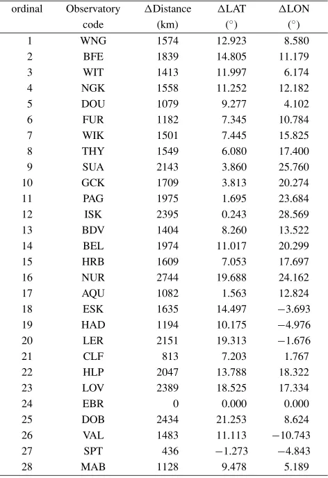
In Fig. 1, a map of Europe displays the positions of the magnetic observatories used in this study. Ebro observa-tory (EBR), located in the SW corner of this area has few neighbours. This may lead to problems of representation for phenomena with gradients not aligned to the main axis of the distribution.

(2)

1188 J. J. CURTO AND S. MARSAL: QUALITY CONTROL OF EBRO MAGNETIC OBSERVATORY USING MOMENTARY VALUES

Table 1. Magnetic observatories used in this study with their position relative to EBR.

ordinal Observatory Distance LAT LON

code (km) (◦) (◦)

1 WNG 1574 12.923 8.580

2 BFE 1839 14.805 11.179

3 WIT 1413 11.997 6.174

4 NGK 1558 11.252 12.182

5 DOU 1079 9.277 4.102

6 FUR 1182 7.345 10.784

7 WIK 1501 7.445 15.825

8 THY 1549 6.080 17.400

9 SUA 2143 3.860 25.760

10 GCK 1709 3.813 20.274

11 PAG 1975 1.695 23.684

12 ISK 2395 0.243 28.569

13 BDV 1404 8.260 13.522

14 BEL 1974 11.017 20.299

15 HRB 1609 7.053 17.697

16 NUR 2744 19.688 24.162

17 AQU 1082 1.563 12.824

18 ESK 1635 14.497 −3.693

19 HAD 1194 10.175 −4.976

20 LER 2151 19.313 −1.676

21 CLF 813 7.203 1.767

22 HLP 2047 13.788 18.322

23 LOV 2389 18.525 17.334

24 EBR 0 0.000 0.000

25 DOB 2434 21.253 8.624

26 VAL 1483 11.113 −10.743

27 SPT 436 −1.273 −4.843

28 MAB 1128 9.478 5.189

2. Procedure

2.1 Analysis of long term trends

For each magnetic element of each observatory we have made use of the monthly means of the momentary values at 02:00 UT reported by Niemegk. With this data, the differ-ences have been calculated by subtracting each participating observatory mean from the respective mean Ebro value:

e= eEBR− eXXX (1)

where eEBR and eXXX are the monthly means of the

momentary values for the “e” magnetic element, and XXX

stands for the 3 letter IAGA code of a magnetic observatory.

The temporal evolution ofeover ﬁve years is shown in

Fig. 2 where, in order to facilitate the comparison, traces have been normalised to an artiﬁcial offset so they start in a common place.

We observe the following traits:

- efor each observatory has a different gradient due to

its individual secular variation.

- For a given magnetic effect, similar peaks appear si-multaneously in several observatories, in particular

those of theZcomponent. Looking in detail: some of

them are magniﬁed at subauroral observatories (Nur-mij¨arvi (NUR), Lovo (LOV), Dombas (DOB) and Ler-wick (LER)); whereas in lower latitude observato-ries (San Pablo-Toledo (SPT)) or western longitudes

Fig. 1. Magnetic observatories over Europe used in this study.

(Valentia (VAL)) these peaks appear with an opposite sense. These phenomena must be linked to processes such as magnetospheric disturbances, ring current, or others.

- Observatories in the Ebro neighbourhood such as Chambon-la-Foret (CLF), L’Aquila (AQU), or San Pablo-Toledo (SPT) in most cases show relatively small slopes.

- There are anomalous traces which don’t correlate with their neighbouring observatories. This is the case of

Istanbul-Kandilli (ISK) for 1997 for theHandZ

com-ponents, Tihany (THY) for 1998, which presents a

jump inD, H andZ components, and ﬁnally Surlari

(SUA) for 2000 in D and for 2001 in D, H and Z.

The magnetic elements of these observatories for the mentioned years should not be taken into consideration in the statistics. Secular variation has a large spatial scale because its source is far away from the stations as compared with the distance between neighbouring ob-servatories, so large differences between them should be considered as anomalous values and hence disre-garded.

Traces ofe follow radial lines and there are no

evi-dences of global jumps or bending, which would point to EBR malfunction.

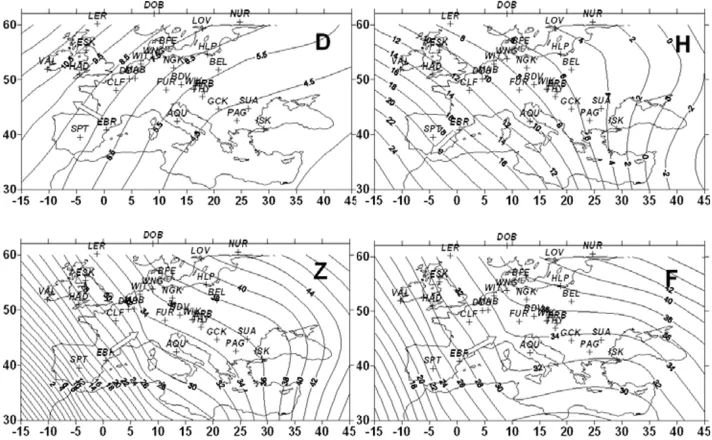
Secular variation (SV) can be expressed with models (Parkinson, 1983; Bloxham and Gubbins, 1985). One of the most important models of SV is the International Geomag-netic Reference Field (IGRF) (Macmillan and Maus, 2005). It is sponsored by IAGA and is kept updated by a continu-ous effort of many researchers. Maps of Europe showing isolines of SV based on the IGRF model for Declination, Horizontal intensity, Vertical intensity and Total Force for 2000 are displayed in Fig. 3.

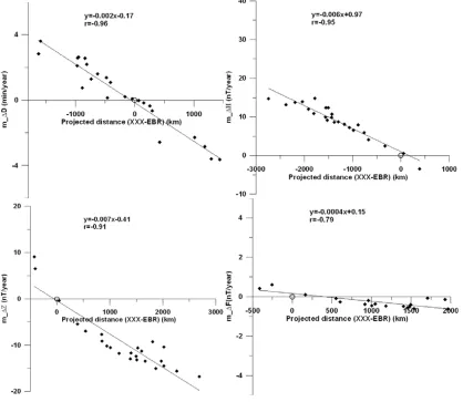
In order to evaluate to what extent the slopes found in Fig. 2 represent secular variation, and knowing the pre-ferred direction of variation of SV according to the IGRF model, we now take as the binning parameter the projection of the distance along the directions marked by the gradient of the SV (big arrows in Fig. 3). Results are displayed in

Fig. 4. Correlation coefﬁcients (r) indicate a good linear

(3)

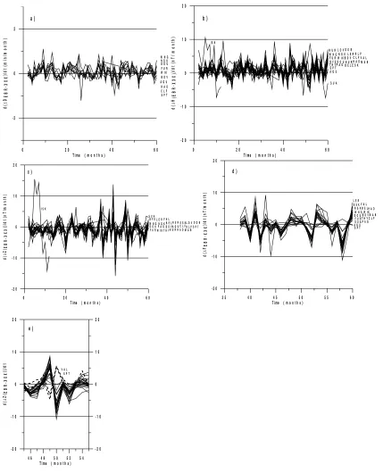
Fig. 2. Temporal variation of the differences between EBR and other observatories (e) for the magnetic components; a)D, b)H, c)Z, and d)F.

Fig. 3. Secular variation of declination, horizontal intensity, vertical intensity and total force for 2000, based on the IGRF model. Units for the isolines are nT/year forH,ZandFand min/year forD. Big arrows represent the main direction of the gradient in the EBR region.

Some points departing from the ﬁt could announce some small malfunctions in that observatory or that the projec-tion of their coordinates done accordingly to the local gra-dient at EBR should not be valid there, a probable cause

for observatories located far away from EBR. This could

be observed in F component, where the magnitude of the

correlation coefﬁcient,r, is lower.

(4)

Fig. 4. Slope versus projected distance forD(upper-left),H(upper-right),Z(bottom-left) andF(bottom-right).

Fig. 5. Some cases of magnetic differences (left) and the appearance of their temporal derivative (right). 1) SV, 2) step due to the introduc-tion of a ferromagnetic object in the neighbourhood of the absolute hut or electronic or mechanical jumps in the standards, 3) isolated anoma-lous value, 4) reallocation of the absolute magnetometer or progressive un-levelling, 5) magnetization or magnet ageing of the sensor.

time ofecan be plotted. The expected slope due to

differ-ences of SV between EBR and another observatory would then be represented as a horizontal line (Fig. 5(1)). A step in EBR would produce here a peak (triangle function) appear-ing simultaneously in all traces (Fig. 5(2)). An anomalous

value would produce a double peak (up-and-down or down-and-up) (Fig. 5(3)). A change in tendency (slope) in EBR would be represented here as a step function in most of the lines (Fig. 5(4)) and, ﬁnally, an acceleration in EBR would be represented here as a continuous slope (Fig. 5(5)).

Traces of the temporal derivative of the differences be-tween Ebro and the other observatories are plotted in Fig. 6. None of the long term malfunctions appear here in any element. However, there are some double peaks

(up-and-down) (e.g. in Z component) which would correspond

to punctual anomalous values. Again, careful inspection shows that those stations to the East of Ebro (CLF, AQU, etc.) systematically have different peak senses from those to the West (SPT, VAL) (Fig. 6(e)). Many of these phe-nomena may be related to natural noise due to non-quiet magnetic conditions, such as ionospheric local meridional currents closing a global circuit, or as a result of anoma-lous magnetic transient variations related to the presence of conductivity heterogeneities in the crust and/or lithosphere.

2.2 Analysis of the coherence of short term variations

(5)

Fig. 6. Derivative of the differences between Ebro and the other observatories for a)D, b)H, c)Zand d)F. e) Detail of Fig. 6(c) showing a double peak. Most of the observatories to the East of EBR have an up-to-down sense, whereas Western observatories (SPT, VAL) present the opposite sense.

(sudden storm commencements (SSC), substorms) (Parkin-son, 1983), and their manifestation sometimes follow irreg-ular patterns.

2.2.1 Test of coherence To check the response of Ebro observatory to “short term variations” in relation to those of the network, another analysis can be performed

us-ing the standard deviation (σ) of the differences of the

mag-netic elements between Ebro and each one of the remaining observatories (Schulz and Gentz, 1998). This will provide the degree of representation of Ebro observatory within the network.

Taking the monthly means of the differences computed in

the previous section, by way of ﬁrst order regression mod-els estimated from the ﬁve neighbouring year values secu-lar variation (SV) is removed, one can evaluate the annual

standard deviation ofefor each observatory (σ e).

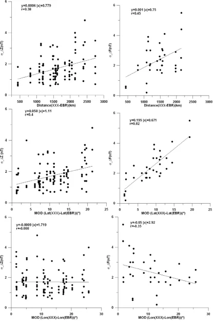
Fig-ures 7(a) and 7(b) showσ eversus absolute value of

dis-tance, longitude or latitude relative to EBR. Again a linear ﬁt can be established as:

σ e(x)=A+B∗|x| (2)

wherexis either distance, latitude or longitude difference

(6)

Fig. 7(a). σ D(left) andσ H(right) against distance and absolute value of latitude and longitude with respect to Ebro. Open circles are neglected points belonging to subauroral observatories with disturbedDcomponent.

an extrapolation is made in order to evaluate the value cor-responding to the reference observatory (in our case, Ebro).

Let us deﬁne Ebro∗as a virtual observatory whose

measure-ments are obtained by extrapolation of the values from other observatories. Ideally, the axis intercept of that linear ﬁt

should be zero, because standard deviation of Ebro∗-Ebro

should be nil. But in fact the virtual measurement Ebro∗

has close characteristics to Ebro but not the same response. Thus different response to latitudinal or longitudinal pro-cesses originated in the auroral zone or in the equatorial zone would affect this term.

(7)

Fig. 7(b). σ Z(left) andσ F(right) against distance and absolute value of latitude and longitude with respect to Ebro.

magnetic element with the position variables, the linear

correlation coefﬁcient (r) has been used. Visual inspection

of Fig. 7 makes clear that linear regression has no meaning for the distance in some cases, and deserves discussion in

the other cases. Small values of the intercept should be interpreted as good coherence of the observatory which has been taken as reference with the network (in this case EBR).

(8)

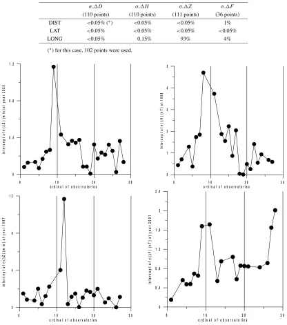
Table 2. Signiﬁcance of the linear correlations according to their probabilities.

σ D σ H σ Z σ F

(110 points) (110 points) (111 points) (36 points)

DIST <0.05% (∗) <0.05% <0.05% 1%

LAT <0.05% <0.05% <0.05% <0.05%

LONG <0.05% 0.15% 93% 4%

(∗) for this case, 102 points were used.

Fig. 8. Examples of annual mean values of the intercepts for the observatories participating in the test. Different components and years are shown. Several clear outlier points appear. Ordinal numbers relate to observatories in Table 1.

(latitude), describe a good linear ﬁt, while others, asσ H

(longitude) or σ Z (longitude), have a poorer ﬁt. We

conclude thatHandZare not linearly related to longitude,

but are to latitude, hence many disturbances have a north-south dependence rather than east-west.

Due to the peripheral location of EBR observatory with respect to the observatories within the network, the ﬁts are highly dependent on the values of the extreme observato-ries, i.e., both those very close to EBR and those very far

from EBR. This is the case for D, which would produce

even a negative value of the intercept. In general, large intercepts should be interpreted as poor coherency of the observatory with the net, or malfunction of the sensors, as incorrect sensitivity or misalignment. Clearly northern ob-servatories (NUR, DOM, LOV, ESK) are more affected by

magnetospheric activity and especially by the ionospheric currents associated to the FAC’s system. So, large networks are not convenient for this kind of study. Although the Wingst/Niemegk selection of the quiet days is done with care, in years close to the maximum of solar activity, as those on scope here, it is not possible to assure that those

10 days per month are absolutely quiet. For the caseσ D

(distance) we decided not include northern observatories in the ﬁnal set.

In order to choose the right value of the axis intercept and to be able to compare it to the rest of the observatories, it has been computed for each magnetic element. The value of the intercept with the ordinate axis differs according

to which variable was considered. For example, σ H

(9)

1 9 9 6 1 9 9 7 1 9 9 8 1 9 9 9 2 0 0 0 2 0 0 1 2 0 0 2

Fig. 9. Annual mean values of the intercepts ofD,H,ZandFfor Ebro against the corresponding values of the whole network for the quinquennium 1997–2001.

as a function of distance, 1.2 nT when it is expressed as a function of latitude, and 1.4 nT if it is expressed as a function of longitude.

To choose the most representative value for each element we have to consider not only its regression coefﬁcient but

also its probability of occurrence. With N data points,

this is deﬁned as the probability to obtain a correlation

coefﬁcient equal to or greater than that being observed (ro)

if these variables were not really correlated. Of course, the lower the probability, the higher the signiﬁcance of the relationship between both variables is.

Table 2 is obtained by taking into account the number of data points and the correlation coefﬁcient in each case (Taylor, 1982).

Probabilities less than 5% can be considered as cant, while those less 1% can be considered as very signifi-cant. Hence, most of the above relations are signifisignifi-cant.

We can conclude that distance is a good variable in the case of declination and horizontal component, whereas lat-itude is a good variable in the case of vertical component and total field. The intercepts with the ordinate axis having the most significant correlation coefficients are:

σ D(DIST=0)=0.00±0.04 min

σ H(DIST=0)=0.6±0.2 nT

σ Z(LAT=LATEBR)=1.1±0.1 nT

σ F(LAT=LATEBR)=0.7±0.2 nT

The quality of the ﬁts (expressed by their correlation coefﬁcient) is equivalent to the previous one showing a good agreement between the independent techniques used.

2.2.2 Detection of outsiders With this method and taking the distance as the abscissa’s variable, we can detect some anomalous values which considerably deviate from the whole net (Fig. 8), pointing out a necessary revision of these measurements.

2.2.3 Test of the performance of the whole

net-work Evolution of the performance of the network in the

preceding years (1973–1995) was shown by Schulz and Gentz (1998), detailing its increasing improvement. Inter-comparison between observatory and international stan-dards with the use of QHM magnetometers in the seventies and the generalization of the DI-ﬂux magnetometers in the eighties (Bitterly, 1990) contributed to this advance.

Finally, comparison between yearly mean values of the intercepts for Ebro and the intercepts of the whole network are shown in Fig. 9.

Error bars represent twice the standard deviation which includes the 95% of the population as a representation of the majority of the network. Ebro results are always between these limits.

3. Conclusions

There is no evidence of discontinuities or jumps in Ebro magnetic elements for the period 1997–2001. The perfor-mance of the observatory is coherent with that of the nearby European observatories.

(10)

From a given observatory, direct comparison of its values with the mean value of the network is not adequate because there are gradients inside the inter-comparison zone which will give a different value depending on the situation of the set of observatories in the sample.

Sometimes, distance by itself is not the best variable to represent tendencies. Most of the disturbing phenomena: SV, effects of auroral electrojet and ring currents have no radial symmetry but longitudinal or latitudinal distribution. In each case, longitudinal and latitudinal dependences have to be considered.

The selection of the ten quietest days per month does not guarantee that they are free from magnetic contamination from external sources.

Acknowledgments. Authors thank D. Gallart for his assistance in data managing and Dr. H. McCreadie for her language revision. Also they are grateful to Dr. G. Schulz and Dr. H. J. Linthe for their effort to provide these lists of quiet days and compile data from the observatories.

References

Bitterly, J., Declinometre-Inclinometre a Vanne de Flux, Institute de Physique du Globe de Strasbourg, 1990.

Bloxham, J. and D. Gubbins, The secular variation of Earth’s magnetic ﬁeld,Nature,317, 777–781, 1985.

Curto, J. J. and E. Sanclement, Levelling error corrections to D-measurements in DI-ﬂux magnetometers,Contributions to Geophysics & Geodesy. Geophys. Inst. Slov. Acad. Sci.,31, 111–117, 2001. Forbes, A. J., General Instrumentation, inGeomagnetism, edited by J. A.

Jacobs, 51–136, Vol. 1, Academic Press, London, 1987.

Gaya-Piqu´e, L. R. and J. M. Torta,El Observatorio Geomagn´etico de Isla Livingston, Publicaciones del Observatorio del Ebro, Roquetes, 2000. Jankowsky, J. and Ch. Sucksdorff,Guide for magnetic measurements and

observatory practice, IAGA publications, Warsaw, 1996.

Macmillan, S. and S. Maus, International Geomagnetic Reference Field, the third generation,Earth Planets Space,57, 1135–1140, 2005. Marsal, S. and J. M. Torta, An evaluation of the uncertainty associated with

the measurement of the geomagnetic ﬁeld with a D/I ﬂuxgate theodolite,

Meas. Sci. Technol.,18, 2143–2156, 2007.

Parkinson, W. D.,Introduction to Geomagnetism, Elsevier, 1983. Schulz, G. and M. Beblo, Monitoring Geomagnetic Standards by the

com-parison of Momentary Values between European observatories in the past, present and future,VIth IAGA workshop on geomagnetic observa-tory instruments, data acquisition and processing, Dourbes, 1996. Schulz, G. and I. Gentz, Results of the momentary value comparison

between European observatories—a summary of the last two decades,

VIIth IAGA workshop on geomagnetic observatory instruments, data acquisition and processing, Niemegk, 1998.

Stuart, W. F., Earth’s Field Magnetometry,Rep. Prog. Phys., 838–847, 1972.

Taylor, J. R.,An introduction to error analysis, the study of uncertainties in Physical Measurements, University Science Books, Oxford University Press, 1982.